Preface
Prerequisites
My aim is for this book to be self-contained. Therefore, the prerequisites are familiarity with calculus and linear algebra. A physics background is also not required beyond what is typically covered in high school, i.e., some knowledge of Newtonian physics including the three laws of motion, Newton's formula for universal gravitation, and trivial extensions of these concepts. This book is written to be self-contained, so you will not need a separate textbook, especially considering the vast availability of online resources and the steep price of textbooks today. I take care to cover all the necessary material in the book itself. However, for students who prefer reading from multiple sources to reinforce their understanding, I would recommend the following two textbooks for further reading. "Introducing Einstein's Relativity" by Ray d'Inverno and "A First Course in General Relativity" by Bernard Schutz. These were also my two primary references during the writing of this book.
Generative AI Disclosure
Generative AI was used as an assistant for the following purposes.
- To help the author review and make targeted corrections to the text that improve grammar, spelling, mathematical notation, correctness of the underlying physics, $\LaTeX{}$ code, and clarity.
- To help the author generate the JavaScript code for the interactive widgets, which was then reviewed and corrected by the author.
License
This is a free and open source textbook licensed under CC BY-SA 4.0. The source code for the animated widgets used in this book is licensed under GNU GPL v3.

Motivation
This book began out of a desire to create free and accessible resources for learning general relativity in specific and more generally for learning mathematics and theoretical physics. I really appreciate how many open source resources exist today for learning all aspect of computer science, but I have found that the fundamental sciences are currently underserved in this regard. This is unfortunate because I believe that now, more than ever, with higher education becoming unaffordable for the vast majority of people, the need to make the fundamental sciences accessible to everyone is crucial. I hope that this book can be a small step in that direction.
As a secondary goal, this book aims to be as readable as possible. I try to 1) define each term that is used and then use the term consistently throughout the text, 2) help the reader work through the mathematical derivations step by step, 3) try to ensure the explanations are clear, intuitive, and easy to follow even at the risk of being annoyingly verbose. I am a somewhat slow learner and this book is my attempt to write a general relativity textbook in a way that I would have liked to learn it the first time. I was inspired by the writing style of what is perhaps the most well-written mathematics textbook I have ever read, "A Book of Abstract Algebra" by Charles C. Pinter. I try to emulate the style of Dr. Pinter in the writing of this book as much as possible and I hope that the reader finds it as enjoyable to read as I found Dr. Pinter's book to be. Now let us start, dear reader, with some fitting verses from the "poet of the east", Iqbal, and then embark on our journey to understand the universe through a beautiful mathematical model.
There are yet more skies before you too
ترے سامنے آسمان اور بھی ہیں
There are other times and spaces that belong to you too
کہ تیرے زمان و مکاں اور بھی ہیں
Introduction
Modelling The Universe
Newtonian mechanics is a reasonably accurate model for the universe when 1) objects are significantly slower than the speed of light, 2) gravity is weak, and 3) objects are macroscopic. Special relativity is a DLC to the universe's video game for when you get to levels where objects whose velocities approach the speed of light, i.e., constraint 1 is relaxed. General relativity is an expanded DLC where you can play levels that have objects of any velocity and where the effects of gravity are not negligible. In other words, constraints 1 and 2 can be relaxed in General relativity.
On a separate axis, Quantum mechanics extends Newtonian mechanics to objects that need not be macroscopic, relaxing constraint 3. Quantum Field Theory can be used for objects that are not macroscopic and objects whose velocity can approach the speed of light, relaxing both constraint 1 and 3. We do not currently have a unified mathematical model that can be used when all three constraints are relaxed.
| Theory | Approaching speed of light | Strong gravity | Microscopic |
|---|---|---|---|
| Newtonian mechanics | N | N | N |
| Special relativity | Y | N | N |
| General relativity | Y | Y | N |
| Quantum mechanics | N | N | Y |
| Quantum field theory | Y | N | Y |
| Quantum gravity | Y | Y | Y |
Preliminaries
We begin by listing the assumptions of Newtonian mechanics. We define a body to be any physical object with mass. A point particle is a simplification of a body that only has mass but does not have any physical size. We define an event to be a point $(x, y, z)$ in space at time $t$. The universe can then be modelled as one large set of events, similar to how open world video games like Grand Theft Auto or Minecraft model their worlds. An object traces out a path through this set of events as time passes. We call this path the object's worldline. To build intuition, consider a cat confined to a single spatial axis. On the left below we watch the cat move along that axis. On the right we plot each event $(x, t)$ she occupies, with position on the horizontal axis and time on the vertical axis. Notice that the slope of the worldline encodes the cat's speed. Walking tilts the line, running tilts it further toward the horizontal, and standing still draws a perfectly vertical segment. When the cat is standing still, she is at rest in space, yet she keeps advancing through time.
Any object that can measure time and measure distance is an observer. You can think of observers as video game characters who can perceive the world around them, e.g., they carry a clock and a measuring stick. The model of the universe constructed using Newtonian mechanics assumes that time is absolute. More concretely, any two observers will always agree about the time of an event, regardless of their relative motion, assuming the clocks they use to measure time are properly synchronized. A coordinate system is an origin and a set of axes. To identify the position of an event, an observer needs to choose a coordinate system. A frame of reference is an observer's chosen coordinate system and chosen clock. Two observers are in the same frame of reference when 1) their clocks are synchronized, 2) they have the same coordinate system, and 3) they are not in motion relative to one another, i.e., their velocity relative to each other is zero. For any event, two observers in the same frame of reference will agree on all four coordinates $(x, y, z, t)$.
Now let's relax assumption 3 and assume that the observers are in motion relative to one another. A coordinate system stays at rest with respect to the observer who sets it up, so when the two observers move relative to each other, a coordinate system at rest for one of them is moving for the other. They can therefore no longer share a single coordinate system, and each observer now uses their own. The two observers will continue to agree on the time $t$ of any event. However, even in Newtonian mechanics, they will no longer agree on the spatial coordinates $(x, y, z)$.
We define an inertial frame of reference to be a frame of reference in which an object with no net force acting on it remains at rest or moves with constant velocity. Consider two inertial frames of reference $S$ and $S^{\prime}$. In Newtonian mechanics, we can transform coordinates from $S$ to $S^{\prime}$ and vice versa using a Galilean transformation. Assume $S$ and $S^{\prime}$ are in standard configuration, i.e., their axes are parallel, their origins coincide at $t = t^{\prime} = 0$, and $S^{\prime}$ moves with constant velocity $v$ along the positive $x$-axis of $S$. This is illustrated in the image below.
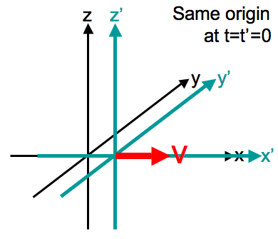
Let $(x, y, z, t)$ be the coordinates of an event in frame $S$ and $(x^{\prime}, y^{\prime}, z^{\prime}, t^{\prime})$ be the coordinates of the same event in frame $S^{\prime}$. The Galilean transformation equations to convert the coordinates of $S$ to the coordinates of $S^{\prime}$ are \[ \begin{aligned} x^{\prime} &= x - vt \\ y^{\prime} &= y \\ z^{\prime} &= z \\ t^{\prime} &= t \end{aligned} \]
Newtonian Mechanics
The Preliminaries section covered the kinematics of Newtonian mechanics which model how an observer assigns coordinates to events. We now turn to the dynamics of Newtonian mechanics which model how forces change the motion of a body. Newton captured the dynamics in three laws. We have already met the first law. Our definition of an inertial frame says that a body with no net force acting on it stays at rest or moves with constant velocity. This is called Newton's first law. We set out the remaining two laws below. Note that special relativity revises the Newtonian laws of motion once we account for the constancy of the speed of light. We will return to the laws of motion when we build relativistic mechanics later in the book.
Every body resists a change in its motion. We call the resistance the body's inertia. The mass of a body is a number $m$ that measures the body's inertia. A body with a larger mass resists a change in its motion more strongly. Assume a body of mass $m$ moves with velocity $v$. We define the body's linear momentum $p$ to be the product of the body's mass, $m$, and the body's velocity, $v$, \begin{equation}\label{eq:linear-momentum} p = m v \end{equation}
A force is a push or a pull that changes the motion of a body. Newton's second law states that the force on a body equals the rate of change of its linear momentum. Formally, \begin{equation}\label{eq:newtons-second-law} F = \frac{dp}{dt} = \frac{d(mv)}{dt} \end{equation} When the mass of the body stays constant, the force is the mass times the acceleration $a = dv/dt$, \[ F = m \frac{dv}{dt} = m a \]
Newton's third law states that to every action there is an equal and opposite reaction. In other words, when one body exerts a force on a second body, the second body exerts a force of equal magnitude and opposite direction on the first. Writing $F_{1}$ for the force on the first body and $F_{2}$ for the force on the second, the third law reads $F_{1} = -F_{2}$.
Newton's laws introduce force and mass as new quantities. How do we measure these two quantities, though? Consider two bodies isolated from every other influence. The only forces present are then the ones the two bodies exert on each other. By the third law the two forces are equal and opposite. The accelerations of the two bodies therefore satisfy $m_{1} a_{1} = -m_{2} a_{2}$, where $a_{1}$ and $a_{2}$ are the accelerations of the first and second body. We fix one body as a standard and assign it unit mass. The relation then fixes the mass of any other body from the two measured accelerations.
We now track the momentum of a system of many particles. Consider a system of $n$ particles. Let the $i$th particle have constant mass $m_{i}$ and velocity $v_{i}$. Its linear momentum is $p_{i} = m_{i} v_{i}$. Let $F_{i}$ be the total force on the $i$th particle. By the second law, $F_{i} = dp_{i}/dt$. The total force on the $i$th particle splits into two parts. The external force $F_{i}^{\text{ext}}$ is the force from sources outside the system. The internal force $F_{ij}$ is the force on the $i$th particle from the $j$th particle. We set $F_{ii} = 0$ since a particle exerts no force on itself. The total force on the $i$th particle is the sum \[ F_{i} = F_{i}^{\text{ext}} + \sum_{j=1}^{n} F_{ij} \]
We define the total linear momentum of the system to be $P = \sum_{i=1}^{n} p_{i}$. Summing the second law over every particle gives \[ \frac{dP}{dt} = \sum_{i=1}^{n} \frac{dp_{i}}{dt} = \sum_{i=1}^{n} F_{i} = \sum_{i=1}^{n} F_{i}^{\text{ext}} + \sum_{i=1}^{n} \sum_{j=1}^{n} F_{ij} \] The third law pairs each internal force with an equal and opposite partner, $F_{ij} = -F_{ji}$. The double sum therefore vanishes. Writing $F^{\text{ext}} = \sum_{i=1}^{n} F_{i}^{\text{ext}}$ for the total external force, we are left with \[ \frac{dP}{dt} = F^{\text{ext}} \]
An isolated system is a system with no external force. Setting $F^{\text{ext}} = 0$ in the relation $dP/dt = F^{\text{ext}}$ gives $dP/dt = 0$. The total linear momentum therefore stays constant in time. Writing $P_{\text{initial}}$ and $P_{\text{final}}$ for the total linear momentum at an earlier and a later time, we have \begin{equation}\label{eq:conservation-of-momentum} P_{\text{initial}} = P_{\text{final}} \end{equation} The result is the conservation of linear momentum. We gave the argument for motion along a single axis. The same argument applies to each spatial direction on its own.
Newton also gave a law for one specific force, the gravitational attraction between two bodies. Newton's universal law of gravitation states that two bodies attract each other with a force proportional to the product of their masses and inversely proportional to the square of the distance between them. For two bodies of mass $m_{1}$ and $m_{2}$ separated by a distance $r$, the force on each body has magnitude \begin{equation}\label{eq:universal-gravitation} F = G \frac{m_{1} m_{2}}{r^{2}} \end{equation} The force on each body points from that body toward the other body. The constant $G$, with an approximate value of $6.67 \times 10^{-11}$ in SI units, is the Newtonian gravitational constant. The next section, special relativity, describes bodies and light in the absence of gravitation. We therefore set the gravitational force aside until we reach general relativity, where a new and exciting theory of gravity replaces the universal law of gravitation from Newtonian mechanics.
Special Relativity
The special theory of relativity is derived from the following two postulates.
- All observers in inertial frames of reference observe the same laws of physics.
- All observers in inertial frames of reference measure the same speed of light in a vacuum.
We will use Bondi's k-calculus approach to understand special relativity here, which is also followed by D'Inverno's text. Let $A$ and $B$ be two observers in inertial frames of reference. Assume $A$ is at rest and $B$ is moving away from $A$ with constant velocity. Assume the universe in which $A$ and $B$ exist only has a single spatial dimension along with the usual time dimension. Therefore, it is sufficient to consider only the $x$ and $t$ coordinates for a given object. Let $A$ send a series of light signals to $B$ at regular intervals of time $T$ as measured by $A$'s clock. Let $T^{\prime}$ be the interarrival time between the light signals as measured by $B$'s clock. We assume $T^{\prime} = kT$. See the left figure below for an illustration of this setup. The k-factor is defined as the ratio of the time interval between the reception of two consecutive signals by $B$ to the time interval $T$ between the emission of two consecutive signals by $A$, i.e., the same $k$ from $T^{\prime} = kT$. The k-factor is a function of the relative velocity between $A$ and $B$.
Consider a light signal sent by $A$ at time $t = T$ according to $A$'s clock and received by $B$ at time $t^{\prime} = T^{\prime} = kT$ according to $B$'s clock. Assume the light signal is reflected back to $A$ by $B$ at event $P$. Since $B$ reflects the signal at the moment it receives it, event $P$ occurs at time $T^{\prime} = kT$ on $B$'s clock. Applying the k-factor again to the return trip, $A$ receives the reflected signal at time $kT^{\prime} = k^2T$ on $A$'s clock. This is illustrated in the right figure above. According to $A$'s clock, the light signal was sent at $t_{1} = T$ and received back at $t_{2} = k^2T$. Therefore, on $A$'s clock, the time coordinate of event $P$ is the average of $t_{1}$ and $t_{2}$, i.e., \[ t = \frac{t_{2} + t_{1}}{2} = \frac{k^2T + T}{2} = \frac{(k^2 + 1)T}{2} \] The $x$ coordinate of event $P$ in $A$'s frame is the distance traveled by the light signal from $A$ to $B$, which is \[ x = \frac{t_{2} - t_{1}}{2} = \frac{k^2T - T}{2} = \frac{(k^2 - 1)T}{2} \] We can use this to find the velocity of $B$ relative to $A$ as measured by $A$'s clock, which is \[ v = \frac{x}{t} = \frac{(k^2 - 1)T/2}{(k^2 + 1)T/2} = \frac{k^2 - 1}{k^2 + 1} \] We can now use this to find the k-factor as a function of the relative velocity $v$ between $A$ and $B$, which is \begin{equation}\label{eq:k-factor-velocity} k = \sqrt{\frac{1 + v}{1 - v}} \end{equation}
Now consider a setup identical to the one above, except with a third observer $C$ also moving away from $A$ with constant velocity. Let $k_{AB}$ be the k-factor between $A$ and $B$, and let $k_{AC}$ be the k-factor between $A$ and $C$. Let $k_{BC}$ be the k-factor between $B$ and $C$. From the way we defined the k-factor, we can see that $k_{AC} = k_{AB}k_{BC}$, i.e., the k-factors multiply. We can also compose velocities using equation \eqref{eq:k-factor-velocity} to find the velocity of $C$ relative to $A$ as a function of the velocities of $B$ and $C$ relative to $A$ and $B$, respectively. \begin{equation}\label{eq:velocity-composition} v_{AC} = \frac{v_{AB} + v_{BC}}{1 + v_{AB}v_{BC}} \end{equation}
Einstein's Gedankenexperiment
Two events are simultaneous for an observer when that observer assigns them the same time coordinate. In Newtonian mechanics time is absolute, so two events that are simultaneous for one observer are simultaneous for every observer. In special relativity this no longer holds. Two events that are simultaneous for $A$ need not be simultaneous for $B$ when $B$ is moving relative to $A$. This is known as the relativity of simultaneity.
To demonstrate the relativity of simultaneity, we use a thought experiment attributed to Albert Einstein. Consider a train moving along a straight track with constant velocity $v$ relative to an observer $A$ standing on the bank. Let $B$ be a second observer who sits at the exact center of one of the train's carriages. Assume a light source is fixed at each end of the train's carriage in which $B$ sits. Also assume that the two light sources are programmed to flash at the same time according to $A$. The two light sources are programmed to flash when, from $A$'s frame of reference, $A$ is equidistant from the two ends of the train's carriage. Now, since $A$ is equidistant from the two ends of the train's carriage and light travels at the same speed in both directions, the two flashes reach $A$ together. $A$ therefore concludes that the flashes were emitted simultaneously.
We will now look at the same two flashes from $B$'s frame of reference. Recall that $B$ sits in the center of the train's carriage, i.e., halfway between the two light sources. Therefore, light emitted at the same time in $B$'s frame would reach $B$ together. That is not what happens. As the light travels, the train carries $B$ toward the flash at the front of the carriage and away from the flash at the back. Since the speed of light is the same for every observer, the light from the front reaches $B$ before the light from the back. $B$ is equidistant from the two sources, so the only conclusion $B$ can draw is that the front flash happened before the back flash. Note that both observers, $A$ and $B$, correctly assigned time coordinates using their own clock and their own light signals. We have thus demonstrated that, in Special Relativity's model of the universe, simultaneity is no longer a property of a pair of events on their own. Simultaneity depends on the observer. By adjusting the timing of one flash slightly, we can even arrange for the two events to happen in one order for $A$ and in the opposite order for $B$.
Due to the relativity of simultaneity, we can no longer assume that two observers in relative motion will agree on the time coordinate of an event. Therefore, we need to find new definitions for what it means for an event to happen before another event. Consider an event $P$. We say that an event $Q$ is in the future light cone of $P$ if a light signal emitted at $P$ can reach $Q$. Similarly, we say that an event $Q$ is in the past light cone of $P$ if a light signal emitted at $Q$ can reach $P$. Light forms cones in spacetime because a light signal spreads out as an expanding sphere in space whose radius grows in step with time, so stacking these spheres up the time axis traces out a cone. Since all inertial observers measure the same speed of light, they will all agree on whether an event is in the future or past light cone of another event.
The causal future of an event $P$ consists of all events that can be reached by a signal traveling at or below the speed of light from $P$. Similarly, the causal past of an event $P$ consists of all events that can send a signal traveling at or below the speed of light to $P$. Since light is the fastest signal, the future and past light cones are the boundaries of the causal future and causal past. The elsewhere consists of all events that are outside both the causal past and causal future of $P$. Note that since we assume no object can travel faster than the speed of light, the points in the causal future of an event $P$ are the only points that can be affected by $P$.
Wacky Timekeeping
The proper time of an observer $A$ between two events is the time recorded by $A$'s clock as it moves from one event to the other. Consider an observer $A$ who stays at rest and a second observer $B$ who leaves $A$. Assume $B$ travels away from $A$ at constant speed, and then $B$ turns around and returns to $A$. When $B$ gets back, $B$'s clock has recorded less proper time than $A$'s clock. In other words, $B$ has aged less than $A$. This result is known as the clock paradox or the twin paradox.
To understand this better, let us replace observer $B$ with two inertial observers $C$ and $D$. Let $C$ move away from $A$ at speed $v$, and let $D$ move toward $A$ at the same speed $v$. $A$ and $C$ meet at event $O$, where they both set their clocks to zero. $C$ travels outward and meets $D$ at event $P$, at which point $C$'s clock reads $T$. At this meeting $D$ sets its clock to $T$, so that $C$ followed by $D$ behaves like a single traveler who goes out and comes back, reading $T$ at the time when the traveler turns around. $D$ continues inward and meets $A$ at event $Q$. Between $O$ and $Q$, the traveling clocks record a total time of $2T$.
We now find the time $A$ records between $O$ and $Q$ using the k-factor. When $C$ and $D$ meet at $P$, they send a light signal back to $A$. Since $C$ is moving away from $A$ and $C$ emitted the signal at time $T$ on $C$'s clock, the k-factor tells us that $A$ receives the signal at time $kT$. The returning observer $D$ approaches $A$ with the opposite velocity, so its k-factor is $k^{-1}$. $A$ meets $D$ at $Q$ a further time $k^{-1}T$ later. The total time $A$ records between $O$ and $Q$ is therefore $(k + k^{-1})T$. For any $k \neq 1$ we have $k + k^{-1} \gt 2$, so $A$ records more time than the $2T$ recorded by $C$ and $D$. Therefore, $A$, the observer who stayed at rest, ages more than the travelling observers $C$ and $D$.
Why can we not reverse the argument and treat $A$ as the traveler who ages less? The three-observer version already contains the answer. The $2T$ was measured by two different inertial observers, $C$ and $D$, not by a single one. To make it a single traveler, that traveler would have to turn around at $P$, and turning around means accelerating. The traveler therefore does not remain in one inertial frame, while $A$ does. The two situations are not symmetric, so there is no matching argument that makes $A$ the younger one. In the model of the world described by Newtonian mechanics, time was absolute. The thought experiment above demonstrates that in special relativity, time is not absolute. Similar to the way distance is dependent on the route taken by an object, in special relativity time is also dependent on the route taken by an object.
Booster Pack
Recall in the preliminaries section we defined the Galilean transformation to convert coordinates from one inertial frame to another. We now derive the special relativity version of the Galilean transformation, known as the Lorentz transformation or the Lorentz boost. Assume $S$ and $S^{\prime}$ are inertial frames of reference in standard configuration. Recall that standard configuration means the axes of $S$ and $S^{\prime}$ are parallel, their origins coincide at $t = t^{\prime} = 0$, and $S^{\prime}$ moves with constant velocity $v$ along the positive $x$-axis of $S$. Consider an event $P$ with coordinates $(x, y, z, t)$ in $S$ and coordinates $(x^{\prime}, y^{\prime}, z^{\prime}, t^{\prime})$ in $S^{\prime}$. We can use the k-factor to find the relationship between the coordinates of $P$ in $S$ and $S^{\prime}$.
A light signal is emitted at time $t_{1}$ according to $S$'s clock to observe event $P$. The light signal is reflected back from $P$ and received at time $t_{2}$ according to $S$'s clock. The time coordinate of event $P$ in $S$ is the average of $t_{1}$ and $t_{2}$, i.e., \[ t = \frac{t_{2} + t_{1}}{2} \] The $x$ coordinate of event $P$ in $S$ is the distance traveled by the light signal from $S$ to $P$, which is \[ x = \frac{t_{2} - t_{1}}{2} \] Recall that since we are using relativistic units, the speed of light is $1$. Therefore, the distance traveled by light is equal to the time taken to travel that distance. These two equations can be solved to find $t_{1}$ and $t_{2}$ in terms of $t$ and $x$, which are \[ t_{1} = t - x, \quad t_{2} = t + x \] Using the same derivations for $S^{\prime}$, we get \[ t_{1}^{\prime} = t^{\prime} - x^{\prime}, \quad t_{2}^{\prime} = t^{\prime} + x^{\prime} \] where $t_{1}^{\prime}$ and $t_{2}^{\prime}$ are the times at which the light signal is emitted and received according to $S^{\prime}$'s clock, respectively. We can now use the k-factor to relate $t_{1}$ and $t_{2}$ to $t_{1}^{\prime}$ and $t_{2}^{\prime}$. The outgoing signal is emitted by $S$ at $t_{1}$ and received by $S^{\prime}$, so $t_{1}^{\prime} = k t_{1}$. The returning signal is emitted by $S^{\prime}$ at $t_{2}^{\prime}$ and received by $S$ at $t_{2}$, so the same rule applied in this direction gives $t_{2} = k t_{2}^{\prime}$. Rearranging the second relation so that both are written for the primed times, we have \[ t_{1}^{\prime} = k t_{1}, \quad t_{2}^{\prime} = k^{-1} t_{2} \] Now, we can use equation \eqref{eq:k-factor-velocity} to find $k$ in terms of $v$, which is \[ k = \sqrt{\frac{1 + v}{1 - v}} \] Replacing $k$ in the equations for $t_{1}^{\prime}$ and $t_{2}^{\prime}$, we have \[ \begin{aligned} t_{1}^{\prime} &= \sqrt{\frac{1 + v}{1 - v}} (t - x) \\ t_{2}^{\prime} &= \sqrt{\frac{1 - v}{1 + v}} (t + x) \end{aligned} \] Similar to $S$, the time coordinate of $P$ in $S^{\prime}$ is the average of $t_{1}^{\prime}$ and $t_{2}^{\prime}$, and the $x^{\prime}$ coordinate is half their difference, i.e., $t^{\prime} = (t_{1}^{\prime} + t_{2}^{\prime})/2$ and $x^{\prime} = (t_{2}^{\prime} - t_{1}^{\prime})/2$. Writing $t_{1}^{\prime}$ and $t_{2}^{\prime}$ back in terms of $k$ to keep the algebra tidy, this is \[ \begin{aligned} t^{\prime} &= \frac{1}{2}\left[k(t - x) + k^{-1}(t + x)\right] \\ x^{\prime} &= \frac{1}{2}\left[k^{-1}(t + x) - k(t - x)\right] \end{aligned} \] Collecting the $t$ and $x$ terms, \[ \begin{aligned} t^{\prime} &= \frac{k + k^{-1}}{2} t - \frac{k - k^{-1}}{2} x \\ x^{\prime} &= \frac{k + k^{-1}}{2} x - \frac{k - k^{-1}}{2} t \end{aligned} \] We now simplify the two combinations of $k$. \[ \begin{aligned} k &= \sqrt{\frac{1 + v}{1 - v}} = \frac{\sqrt{1 + v}}{\sqrt{1 - v}} \\ &= \frac{\sqrt{1 + v}}{\sqrt{1 - v}} \times \frac{\sqrt{1 + v}}{\sqrt{1 + v}} = \frac{1 + v}{\sqrt{(1 - v)(1 + v)}} \\ &= \frac{1 + v}{\sqrt{1^2 - v^2}} = \frac{1 + v}{\sqrt{1 - v^2}} \end{aligned} \] Using the same method, we can also find $k^{-1}$ in terms of $v$, which is \[ \quad k^{-1} = \sqrt{\frac{1 - v}{1 + v}} = \frac{1 - v}{\sqrt{1 - v^2}} \] Now we use these in the two combinations of $k$ \[ k + k^{-1} = \frac{(1 + v) + (1 - v)}{\sqrt{1 - v^2}} = \frac{2}{\sqrt{1 - v^2}} \] and \[ k - k^{-1} = \frac{(1 + v) - (1 - v)}{\sqrt{1 - v^2}} = \frac{2v}{\sqrt{1 - v^2}} \] Dividing each by $2$, the two combinations of $k$ are \[ \frac{k + k^{-1}}{2} = \frac{1}{\sqrt{1 - v^2}} \] and \[ \frac{k - k^{-1}}{2} = \frac{v}{\sqrt{1 - v^2}} \] Let $\gamma = 1/\sqrt{1 - v^2}$. Also recall that the $y$ and $z$ coordinates are unchanged in the standard configuration. This finally gives us the Lorentz transformation to convert coordinates from $S$ to $S^{\prime}$. \begin{equation}\label{eq:lorentz} \begin{aligned} t^{\prime} &= \gamma(t - vx) \\ x^{\prime} &= \gamma(x - vt) \\ y^{\prime} &= y \\ z^{\prime} &= z \end{aligned} \end{equation}
We have worked in relativistic units, where $c = 1$. Restoring the factors of $c$ by dimensional analysis, the $vx$ term in the equation for $t^{\prime}$ becomes $vx/c^2$ while the equation for $x^{\prime}$ is unchanged. This gives \begin{equation}\label{eq:lorentz-standard} \begin{aligned} t^{\prime} &= \gamma_{s}\left(t - \frac{v x}{c^2}\right) \\ x^{\prime} &= \gamma_{s}(x - vt) \\ y^{\prime} &= y \\ z^{\prime} &= z \end{aligned} \end{equation} where $\gamma_{s} = \frac{1}{\sqrt{1 - v^2/c^2}}$. It is also convenient to write the transformation as a matrix. Switching back to relativistic units where $c = 1$, we have \[ \begin{bmatrix} t^{\prime} \\ x^{\prime} \\ y^{\prime} \\ z^{\prime} \end{bmatrix} = \begin{bmatrix} \gamma & -\gamma v & 0 & 0 \\ -\gamma v & \gamma & 0 & 0 \\ 0 & 0 & 1 & 0 \\ 0 & 0 & 0 & 1 \end{bmatrix} \begin{bmatrix} t \\ x \\ y \\ z \end{bmatrix} \] This matrix form is helpful because it generalizes when we later describe spacetime using tensors. Note that the Lorentz transformation can also be derived from first principles, without the k-calculus approach. A free particle, i.e., a particle subject to no forces, moves with constant velocity in every inertial frame. A transformation that takes constant-velocity motion to constant-velocity motion must be linear, which fixes its form up to a few constants. Requiring that the speed of light be the same in both frames then determines those constants and gives the Lorentz transformation.
In the model of the universe described by Newtonian mechanics, time is invariant, i.e., every observer agrees on the time coordinate of an event. Similarly, every observer agrees on the distance between two events measured at the same time, \[ \begin{aligned} \sigma^2 &= (x_1 - x_2)^2 + (y_1 - y_2)^2 \\ &\quad + (z_1 - z_2)^2 \end{aligned} \] The Lorentz transformation deconstructs both of these ideas, since it mixes the time and space coordinates together. However, we can still define a quantity that remains invariant under the Lorentz transformation. To define it, we need to treat time and space as a single four-dimensional continuum called spacetime. For two events $(t_1, x_1, y_1, z_1)$ and $(t_2, x_2, y_2, z_2)$, we define the square of the spacetime interval between them to be \begin{equation}\label{eq:interval} \begin{aligned} s^2 &= (t_1 - t_2)^2 - (x_1 - x_2)^2 \\ &\quad - (y_1 - y_2)^2 - (z_1 - z_2)^2 \end{aligned} \end{equation} We always work with the square $s^2$, since the interval $s$ itself is only defined when the right-hand side is not negative. The spacetime interval is also just referred to as the interval.
Now we show that every inertial observer assigns the same interval to a pair of events. Let $S$ and $S^{\prime}$ be two observers in the standard configuration. Let $P$ be an event with coordinates $(x, y, z, t)$ as measured by $S$. According to $S$, the interval between event $P$ and the origin is $s^2 = t^2 - x^2 - y^2 - z^2$. We compute the same quantity in $S^{\prime}$ using equation \eqref{eq:lorentz}. Since $y^{\prime} = y$ and $z^{\prime} = z$, only the $t$ and $x$ terms can change, so we focus on those. \[ t^{\prime 2} - x^{\prime 2} = \gamma^2 (t - vx)^2 - \gamma^2 (x - vt)^2 \] Expanding the two squares, the cross terms $-2vtx$ cancel, and we are left with \[ \begin{aligned} t^{\prime 2} - x^{\prime 2} &= \gamma^2\left[(t^2 + v^2 x^2) - (x^2 + v^2 t^2)\right] \\ &= \gamma^2 (1 - v^2)(t^2 - x^2) \end{aligned} \] Since $\gamma = 1/\sqrt{1 - v^2}$, we have $\gamma^2 (1 - v^2) = 1$. This simplifies $t^{\prime 2} - x^{\prime 2}$ to $t^2 - x^2$. Adding the unchanged $y$ and $z$ terms gives $s^{\prime 2} = s^2$. The interval is therefore the same in every inertial frame. We say the interval is invariant under the Lorentz transformation.
So far we have only checked the interval between an event and the origin. To see that the interval between any two events $P_1 = (t_1, x_1, y_1, z_1)$ and $P_2 = (t_2, x_2, y_2, z_2)$ is also invariant, we can write their coordinate differences as $\Delta t = t_1 - t_2$, $\Delta x = x_1 - x_2$, $\Delta y = y_1 - y_2$, and $\Delta z = z_1 - z_2$. The square of the interval between $P_1$ and $P_2$ is \[ s^2 = \Delta t^2 - \Delta x^2 - \Delta y^2 - \Delta z^2 \] The Lorentz transformation is a linear transformation in the linear algebra sense, which means subtracting the transformation of $P_2$ from the transformation of $P_1$ gives us the same expression as the transformation of $P_1$ but acting on the coordinate differences between $P_1$ and $P_2$. For example, consider the time coordinate. The Lorentz transformation gives \[ \begin{aligned} \Delta t^{\prime} &= t_1^{\prime} - t_2^{\prime} \\ &= \gamma(t_1 - v x_1) - \gamma(t_2 - v x_2) \\ &= \gamma(\Delta t - v\,\Delta x) \end{aligned} \] and the same steps for the other coordinates give $\Delta x^{\prime} = \gamma(\Delta x - v\,\Delta t)$, $\Delta y^{\prime} = \Delta y$, and $\Delta z^{\prime} = \Delta z$. These are identical to equation \eqref{eq:lorentz} but with the coordinates replaced by the differences in coordinates. Therefore, the invariance calculation for two events is identical to the invariance calculation between an event and the origin. It follows that the interval between any two events is invariant, similar to the interval of an event as measured from the origin.
The spacetime interval replaces the two separate absolute quantities of Newtonian mechanics, i.e., absolute time and Euclidean distance. The sign of $s^2$ tells us how two events are causally related. When $s^2 \gt 0$, we define the interval to be timelike. For timelike intervals, one event lies inside the other's light cone, i.e., a single observer $A$ travelling slower than light can be present at both. $A$ records $\sqrt{s^2}$ as the proper time between the two events. When $s^2 = 0$ the interval is null. For null intervals, the two events lie on each other's light cone. The only thing that can connect two events in a null interval is a light signal. A null interval has equal spatial and temporal separation, so connecting the two events requires travelling at exactly the speed of light. Light travels at exactly this speed, while any massive object travels strictly slower, so only a light signal can bridge a null interval. Finally, when $s^2 \lt 0$, the interval is spacelike. For a spacelike interval, each event lies in the other event's elsewhere. Therefore, no observer can be present at both events.
A four-dimensional spacetime equipped with the spacetime interval is called Minkowski spacetime. Special relativity is essentially the study of physics in Minkowski spacetime. For two events separated by an infinitesimal coordinate difference, the interval becomes \[ \mathrm{d}s^2 = \mathrm{d}t^2 - \mathrm{d}x^2 - \mathrm{d}y^2 - \mathrm{d}z^2 \] This infinitesimal form of the spacetime interval can be carried over into general relativity. We will discuss this in more detail later.
A Slice of Group Theory
This section is a short detour, included because it is fun and because the same idea returns later. The Lorentz transformations we just derived have a tidy algebraic structure. They form a group. A group is a set $G$ together with a way of combining any two of its elements, written $a \star b$, that obeys four rules.
- Closure. For any $a$ and $b$ in $G$, the combination $a \star b$ is also in $G$.
- Associativity. For any $a$, $b$, and $c$ in $G$, we have $(a \star b) \star c = a \star (b \star c)$.
- Identity. There is an element $e$ in $G$ such that $e \star a = a \star e = a$ for every $a$ in $G$.
- Inverse. For every $a$ in $G$ there is an element $a^{-1}$ in $G$ such that $a \star a^{-1} = a^{-1} \star a = e$.
A familiar example is the set of integers under addition. Adding two integers gives an integer, so closure holds. Addition is associative, the identity is $0$, and the inverse of $n$ is $-n$. An abelian group is any group that also has one additional property, commutativity.
- Commutativity. For any $a$ and $b$ in $G$, we have $a \star b = b \star a$.
Now consider the special Lorentz transformations, i.e., the boosts along the $x$-axis, working in relativistic units where $c = 1$. Each boost is completely determined by the relative velocity, $v$. Therefore, we can denote the boost as $B_v$ where $v$ is the relative velocity. Let $P$ be an event with coordinates $(t, x, y, z)$ in one inertial frame and coordinates $(t^{\prime}, x^{\prime}, y^{\prime}, z^{\prime})$ in another inertial frame moving at velocity $v$ relative to the first. The boost $B_v$ is the linear transformation that takes the coordinates of $P$ in the first frame to its coordinates in the second frame. In matrix form, this is \[ B_v = \begin{bmatrix} \gamma & -\gamma v \\ -\gamma v & \gamma \end{bmatrix}, \quad \gamma = \frac{1}{\sqrt{1 - v^2}} \] Note that $y$ and $z$ are left unchanged. Let $G$ be the set of all such boosts $B_v$. $G$ contains a boost for every velocity $v$ that has magnitude less than the speed of light, i.e., $|v| \lt c$. Consider the operation of composition, i.e., one boost applied after another boost, acting on the elements of $G$. We claim that $G$ forms a group under this operation.
Closure holds because applying $B_v$ followed by $B_{v'}$ is the same as a single boost $B_{v''}$, where $v''$ is given by the velocity composition law from equation \eqref{eq:velocity-composition}. For velocities $v$ and $v'$ along the same axis, the velocity composition law is \[ v'' = \frac{v + v'}{1 + v v'} \] Since $v$ and $v'$ each have magnitude less than the speed of light, so does $v''$, so $B_{v''}$ is again a boost in our set. The identity is the boost with $v = 0$, which leaves every coordinate unchanged. The inverse of $B_v$ is $B_{-v}$, since boosting by $v$ and then by $-v$ returns us to where we started. We can see this below. \[ \begin{aligned} B_v B_{-v} &= \begin{bmatrix} \gamma & -\gamma v \\ -\gamma v & \gamma \end{bmatrix} \begin{bmatrix} \gamma & \gamma v \\ \gamma v & \gamma \end{bmatrix} \\[4pt] &= \begin{bmatrix} \gamma^2 - \gamma^2 v^2 & \gamma^2 v - \gamma^2 v \\ -\gamma^2 v + \gamma^2 v & \gamma^2 - \gamma^2 v^2 \end{bmatrix} \\[4pt] &= \begin{bmatrix} \gamma^2 (1 - v^2) & 0 \\ 0 & \gamma^2 (1 - v^2) \end{bmatrix} \\[4pt] &= \begin{bmatrix} \dfrac{1 - v^2}{1 - v^2} & 0 \\ 0 & \dfrac{1 - v^2}{1 - v^2} \end{bmatrix} \\[4pt] &= \begin{bmatrix} 1 & 0 \\ 0 & 1 \end{bmatrix} \end{aligned} \] Finally, associativity holds because composing boosts is just multiplying their matrices, and matrix multiplication is associative. The boosts along the $x$-axis therefore form a group. Note that the group is also abelian, since the formula for $v''$ is unchanged when we swap $v$ and $v'$, i.e., $B_{v}B_{v^{\prime}} = B_{v^{\prime}}B_{v}$. Therefore, commutativity also holds.
There is a nicer way to see all of this. We can define the rapidity $\phi$ of a boost by $v = \tanh \phi$. Using $\gamma = \cosh \phi$ and $\gamma v = \sinh \phi$, the boost matrix becomes \[ B_v = \begin{bmatrix} \cosh \phi & -\sinh \phi \\ -\sinh \phi & \cosh \phi \end{bmatrix} \] This is the hyperbolic cousin of an ordinary rotation matrix, so a boost is really a rotation in spacetime through the rapidity $\phi$. Two boosts compose by simply adding their rapidities, $\phi'' = \phi + \phi'$, in the same way that ordinary rotations add their angles.
We have only looked at boosts along a single axis. The full collection of Lorentz transformations, which also allows boosts in any direction together with ordinary spatial rotations, forms a larger group called the Lorentz group. This group is not abelian, since combining boosts along different directions produces a spatial rotation in addition to a boost. We will return to it later.
Length Contraction and Time Dilation
We now use the Lorentz transformation to work out two of its most striking consequences. The first is that a moving object is shorter along its direction of motion than the same object at rest. This is called length contraction.
Consider two inertial frames of reference $S$ and $S^{\prime}$ in the standard configuration. Let's assume a rod is lying along the $x$-axis and at rest in $S^{\prime}$, with its ends at $x_A^{\prime}$ and $x_B^{\prime}$. Since the rod does not move in $S^{\prime}$, the coordinates of the ends of the rod, i.e., $x_A^{\prime}$ and $x_B^{\prime}$, do not change with time. We call the length of the rod in $S^{\prime}$, the frame where it is at rest, the rod's proper length. The proper length for the rod is $\ell_0 = x_B^{\prime} - x_A^{\prime}$. Now we measure the rod in $S$, the frame in which it moves at velocity $v$. In $S$, the ends of the rod move with velocity $v$, so their positions change with time. To get a length for the rod, we must read off both ends at the same time in $S$. This is the key point. A length is the distance between the two ends taken at a single instant, and two observers who disagree about simultaneity disagree about length. Let $S$ read both ends at the same time $t_A = t_B$. Let's denote the length of the rod as measured in $S$ as $\ell$. The length of the rod in $S$ is then $\ell = x_B - x_A$.
The Lorentz transformation in equation \eqref{eq:lorentz} relates the coordinates of each end of the rod in $S$ to its coordinates in $S^{\prime}$. For the end at $x_A^{\prime}$, we have $x_A^{\prime} = \gamma(x_A - v t_A)$. Similarly, for the other end at $x_B^{\prime}$, we have $x_B^{\prime} = \gamma(x_B - v t_B)$. Subtracting the first equation from the second and using $t_A = t_B$, the time terms cancel and we are left with $\ell_0 = x_B^{\prime} - x_A^{\prime} = \gamma(x_{B} - v t_B) - \gamma(x_{A} - v t_A) = \gamma\left[(x_B - x_A) - v(t_B - t_A)\right] = \gamma(x_B - x_A) = \gamma \ell$. Rearranging this to get $\ell$, the length measured in $S$ is \begin{equation}\label{eq:length-contraction} \ell = \frac{\ell_0}{\gamma} = \ell_0 \sqrt{1 - v^2} \end{equation}
Since $\gamma \gt 1$ whenever $v \neq 0$, we have $\ell \lt \ell_0$. This implies that the moving rod is shorter than its rest length by the factor $\sqrt{1 - v^2}$. The rod is longest in its own rest frame, and its measured length shrinks toward zero as $v$ approaches the speed of light, i.e., $v \to c=1$.
Two points are worth stressing. First, nothing is physically squeezing the rod. The contraction comes from the relativity of simultaneity. $S$ and $S^{\prime}$ do not agree on which events happen at the same time, so they do not agree on where the two ends are at a single instant, and therefore they do not agree on the length. Second, length contraction is reciprocal, i.e., it is symmetric between the two frames. We found that a rod at rest in $S^{\prime}$ is measured as shorter by $S$. The same argument with the roles of $S$ and $S^{\prime}$ swapped shows that a rod at rest in $S$ is measured as shorter by $S^{\prime}$, by the same factor $\sqrt{1 - v^2}$. The two measurements do not conflict, since each observer reads off the two ends using their own pair of simultaneous events. Note that there is no length contraction in the directions perpendicular to the direction of the motion, since the Lorentz transformation leaves the $y$ and $z$ coordinates unchanged.
The second striking consequence of the Lorentz transformation is that a moving clock runs slow. The time between two ticks of any given clock is measured to take longer when the clock is moving relative to an observer as compared to when the clock is at rest relative to that observer. This phenomenon is called time dilation. We return again to the two inertial frames of reference $S$ and $S^{\prime}$ in the standard configuration. Consider a clock at rest in $S^{\prime}$. It ticks at two events, which in $S$ have coordinates $(t_1, x_1)$ and $(t_2, x_2)$. Let $T_0$ be the time between the two ticks in $S^{\prime}$, the frame where the clock is at rest. We want the time $T = t_2 - t_1$ between the same two ticks as measured in $S$, where the clock moves at velocity $v$.
Applying the Lorentz transformation in equation \eqref{eq:lorentz} to each tick, \[ \begin{aligned} t_1^{\prime} &= \gamma(t_1 - v x_1) \\ t_2^{\prime} &= \gamma(t_2 - v x_2) \end{aligned} \] The time between the ticks in $S^{\prime}$ is the difference of these, $T_0 = t_2^{\prime} - t_1^{\prime}$. In $S$ the clock moves at velocity $v$, so between the same two ticks, the clock's position in $S$ changes by $x_2 - x_1 = v(t_2 - t_1) = vT$. Subtracting the two equations and using this relation gives, \[ \begin{aligned} T_0 &= \gamma\left[(t_2 - t_1) - v(x_2 - x_1)\right] \\ &= \gamma\left(T - v \cdot vT\right) \\ &= \gamma(1 - v^2)\,T \end{aligned} \] Since $\gamma = 1/\sqrt{1 - v^2}$, we have $\gamma(1 - v^2) = 1/\gamma$. This simplifies our derivation to $T_0 = T/\gamma$. Rearranging to make $T$ the subject of the equation, the time measured in $S$ is \begin{equation}\label{eq:time-dilation} T = \gamma T_0 \end{equation}
Since $\gamma \gt 1$ whenever $v \neq 0$, we have $T \gt T_0$. We have thus shown that the two ticks are farther apart in time as measured in $S$ where the clock is moving at velocity $v$ as compared to $S^{\prime}$, where the clock is at rest. A clock therefore runs at its fastest rate in its own rest frame. The rate of a clock in a frame where it is at rest is called the clock's proper rate. Like length contraction, time dilation is also reciprocal. For example, a clock at rest in $S$ runs slow as measured in $S^{\prime}$, by the same factor $\gamma$.
The result we have derived so far applies to a clock moving at constant velocity. We now consider a clock that accelerates. We define an ideal clock to be a clock whose rate depends only on its instantaneous speed and not on its acceleration. Let's assume that a real clock behaves like an ideal clock. This assumption is called the clock hypothesis. At each moment an accelerating clock has a definite speed $v$. We can split the accelerating clock's motion into short intervals $\mathrm{d}t$ of time in $S$ and apply the time dilation relation \eqref{eq:time-dilation} to each one of these intervals. Over each infinitesimal interval the speed $v$ is effectively constant, and this becomes exact as $\mathrm{d}t \to 0$. Over one such interval the clock advances its own reading by $\sqrt{1 - v^2}\,\mathrm{d}t$. Adding these contributions along the clock's worldline, the total time the clock reads between two events is \begin{equation}\label{eq:proper-time} \tau = \int \sqrt{1 - v^2}\,\mathrm{d}t \end{equation} We defined proper time earlier as the time a clock records between two events. $\tau$ in the equation above is the proper time of the accelerating clock. Equation \eqref{eq:proper-time} shows that the proper time depends on the route the clock takes through spacetime. This route dependence is why the observer who stays at rest in the clock paradox ages more than the traveler. The spacetime interval \eqref{eq:interval} provides an explanation for this. In the interval, the time difference between two events is added while the space differences are subtracted. The proper time a clock records between the events is the spacetime interval measured along the clock's own path. Between two events at the same place, a clock that stays at rest records the most proper time, while a clock that travels out and back records less proper time. Note that for a clock moving at constant velocity, the integral above resolves to $\tau = \sqrt{1 - v^2}\,T = T_0$. This makes sense, since the proper time of a clock moving at constant velocity is the time between two ticks as measured in the clock's rest frame.
Velocity and Acceleration
The Lorentz transformation tells us how the position and time coordinates of an event change between frames. We now ask how a velocity changes between frames. Consider a particle moving through both $S$ and $S^{\prime}$, which stay in the standard configuration with $S^{\prime}$ moving at velocity $v$ along the $x$ axis of $S$. We can write the particle's velocity in $S$ as $(u_x, u_y, u_z)$, where $u_x = \mathrm{d}x/\mathrm{d}t$ and $u_y$ and $u_z$ follow the same pattern. We can also write the particle's velocity in $S^{\prime}$ as $(u_x^{\prime}, u_y^{\prime}, u_z^{\prime})$, where $u_x^{\prime} = \mathrm{d}x^{\prime}/\mathrm{d}t^{\prime}$ and again the other two components follow the same pattern.
Taking differentials of the Lorentz transformation \eqref{eq:lorentz} gives \[ \begin{aligned} \mathrm{d}t^{\prime} &= \gamma(\mathrm{d}t - v\,\mathrm{d}x) \\ \mathrm{d}x^{\prime} &= \gamma(\mathrm{d}x - v\,\mathrm{d}t) \\ \mathrm{d}y^{\prime} &= \mathrm{d}y \\ \mathrm{d}z^{\prime} &= \mathrm{d}z \end{aligned} \] For the component along the direction of motion, we divide $\mathrm{d}x^{\prime}$ by $\mathrm{d}t^{\prime}$ and then divide the numerator and denominator by $\mathrm{d}t$, \[ u_x^{\prime} = \frac{\mathrm{d}x^{\prime}}{\mathrm{d}t^{\prime}} = \frac{\gamma(\mathrm{d}x - v\,\mathrm{d}t)}{\gamma(\mathrm{d}t - v\,\mathrm{d}x)} = \frac{\mathrm{d}x/\mathrm{d}t - v}{1 - v\,\mathrm{d}x/\mathrm{d}t} = \frac{u_x - v}{1 - u_x v} \] For the two components perpendicular to the motion, we divide $\mathrm{d}y^{\prime}$ and $\mathrm{d}z^{\prime}$ by $\mathrm{d}t^{\prime}$ in the same way. The $y$ component is \[ u_y^{\prime} = \frac{\mathrm{d}y^{\prime}}{\mathrm{d}t^{\prime}} = \frac{\mathrm{d}y}{\gamma(\mathrm{d}t - v\,\mathrm{d}x)} = \frac{\mathrm{d}y/\mathrm{d}t}{\gamma(1 - v\,\mathrm{d}x/\mathrm{d}t)} = \frac{u_y}{\gamma(1 - u_x v)} \] and the $z$ component follows identically. Collecting the three components, \begin{equation}\label{eq:velocity-transformation} \begin{aligned} u_x^{\prime} &= \frac{u_x - v}{1 - u_x v} \\ u_y^{\prime} &= \frac{u_y}{\gamma(1 - u_x v)} \\ u_z^{\prime} &= \frac{u_z}{\gamma(1 - u_x v)} \end{aligned} \end{equation} To go from $S^{\prime}$ back to $S$, we swap the primed and unprimed components and replace $v$ with $-v$.
Two features are worth stressing. First, the component $u_x^{\prime}$ along the direction of motion is the velocity-composition law we derived by the k-calculus in equation \eqref{eq:velocity-composition}. Composing the particle's velocity $u_x$ in $S$ with the velocity $-v$ of $S$ relative to $S^{\prime}$ gives exactly $u_x^{\prime} = (u_x - v)/(1 - u_x v)$. Second, the perpendicular components $u_y^{\prime}$ and $u_z^{\prime}$ differ from $u_y$ and $u_z$, even though the perpendicular coordinates satisfy $y^{\prime} = y$ and $z^{\prime} = z$ and do not change at all. A velocity is a coordinate distance divided by a time, and the two frames disagree on the time. Since $\mathrm{d}t^{\prime} \neq \mathrm{d}t$, dividing the same $\mathrm{d}y$ by the two different time intervals gives two different perpendicular velocities.
We define the particle's acceleration in $S$ as $a_x = \mathrm{d}u_x/\mathrm{d}t$, and its acceleration in $S^{\prime}$ as $a_x^{\prime} = \mathrm{d}u_x^{\prime}/\mathrm{d}t^{\prime}$, and we define the perpendicular components the same way. To find how the acceleration along the direction of motion transforms, we start from the inverse of the first line of \eqref{eq:velocity-transformation}, \[ u_x = \frac{u_x^{\prime} + v}{1 + u_x^{\prime} v} \] Taking the differential and using $1 - v^2 = 1/\gamma^2$ gives \[ \mathrm{d}u_x = \frac{1 - v^2}{(1 + u_x^{\prime} v)^2}\,\mathrm{d}u_x^{\prime} = \frac{1}{\gamma^2 (1 + u_x^{\prime} v)^2}\,\mathrm{d}u_x^{\prime} \] We still need $\mathrm{d}t$ in terms of the $S^{\prime}$ quantities. The inverse Lorentz transformation expresses the $S$ coordinates in terms of the $S^{\prime}$ coordinates, and we get it by solving \eqref{eq:lorentz} for $t$ and $x$. Equivalently, since $S$ moves at velocity $-v$ relative to $S^{\prime}$, the inverse has the same form as \eqref{eq:lorentz} with the primed and unprimed coordinates swapped and $v$ replaced by $-v$, \[ \begin{aligned} t &= \gamma(t^{\prime} + v x^{\prime}) \\ x &= \gamma(x^{\prime} + v t^{\prime}) \end{aligned} \] with $y = y^{\prime}$ and $z = z^{\prime}$ unchanged. Taking the differential of the first line gives $\mathrm{d}t = \gamma(\mathrm{d}t^{\prime} + v\,\mathrm{d}x^{\prime})$. Factoring out $\mathrm{d}t^{\prime}$ and using $u_x^{\prime} = \mathrm{d}x^{\prime}/\mathrm{d}t^{\prime}$, \[ \mathrm{d}t = \gamma(\mathrm{d}t^{\prime} + v\,\mathrm{d}x^{\prime}) = \gamma\left(1 + v\,\frac{\mathrm{d}x^{\prime}}{\mathrm{d}t^{\prime}}\right)\mathrm{d}t^{\prime} = \gamma(1 + u_x^{\prime} v)\,\mathrm{d}t^{\prime} \] Dividing $\mathrm{d}u_x$ by $\mathrm{d}t$, the acceleration along the direction of motion is \[ a_x = \frac{\mathrm{d}u_x}{\mathrm{d}t} = \frac{\dfrac{1}{\gamma^2 (1 + u_x^{\prime} v)^2}\,\mathrm{d}u_x^{\prime}}{\gamma(1 + u_x^{\prime} v)\,\mathrm{d}t^{\prime}} = \frac{1}{\gamma^3 (1 + u_x^{\prime} v)^3}\,\frac{\mathrm{d}u_x^{\prime}}{\mathrm{d}t^{\prime}} \] Since $a_x^{\prime} = \mathrm{d}u_x^{\prime}/\mathrm{d}t^{\prime}$, the acceleration along the direction of motion transforms as \begin{equation}\label{eq:acceleration-transformation} a_x = \frac{a_x^{\prime}}{\gamma^3 (1 + u_x^{\prime} v)^3} \end{equation} The two perpendicular components transform in a similar way, each as a linear combination of the components of the acceleration in $S^{\prime}$.
Equation \eqref{eq:acceleration-transformation} says that the acceleration in $S$ depends not only on the acceleration in $S^{\prime}$ but also on the particle's velocity $u_x^{\prime}$ and on the relative speed $v$ of the frames. The value of the acceleration therefore differs from one inertial frame to another, unlike in Newtonian mechanics, where all inertial observers measure the same acceleration. The value of the acceleration is relative in special relativity. Whether the acceleration is zero, though, is not relative. We fix the particle's velocity. Then \eqref{eq:acceleration-transformation} and the two perpendicular formulas turn the acceleration vector $(a_x^{\prime}, a_y^{\prime}, a_z^{\prime})$ in $S^{\prime}$ into the acceleration vector $(a_x, a_y, a_z)$ in $S$ through a linear map, meaning each component of the acceleration in $S$ is a fixed weighted sum of the components of the acceleration in $S^{\prime}$, with the weights set by the velocity. We can write $L$ for this linear map, so $L$ sends $(a_x^{\prime}, a_y^{\prime}, a_z^{\prime})$ to $(a_x, a_y, a_z)$. The map $L$ is invertible, meaning there is a map $L^{-1}$ for which \[ L^{-1}\big(L(a_x^{\prime}, a_y^{\prime}, a_z^{\prime})\big) = (a_x^{\prime}, a_y^{\prime}, a_z^{\prime}) \] for every $(a_x^{\prime}, a_y^{\prime}, a_z^{\prime})$. Here $L^{-1}$ is the acceleration transformation from $S$ to $S^{\prime}$, which we obtain from the formulas above by swapping the primed and unprimed components and replacing $v$ with $-v$. Two consequences follow. The map $L$ is linear, so it sends the zero vector to the zero vector, $L(0,0,0) = (0,0,0)$. The map $L$ is also invertible, so the zero vector is the only vector $L$ sends to $(0,0,0)$. To see this, suppose $L(a_x^{\prime}, a_y^{\prime}, a_z^{\prime}) = (0,0,0)$. Then \[ (a_x^{\prime}, a_y^{\prime}, a_z^{\prime}) = L^{-1}\big(L(a_x^{\prime}, a_y^{\prime}, a_z^{\prime})\big) = L^{-1}(0,0,0) = L^{-1}\big(L(0,0,0)\big) = (0,0,0) \] where the first and last equalities are the defining identity of $L^{-1}$, the second uses the supposition $L(a_x^{\prime}, a_y^{\prime}, a_z^{\prime}) = (0,0,0)$, and the third uses $L(0,0,0) = (0,0,0)$. So the acceleration in $S$ is zero exactly when the acceleration in $S^{\prime}$ is zero. All inertial observers disagree on the value of a particle's acceleration but agree on whether the particle accelerates at all. In this sense acceleration is absolute in special relativity.
We can now compare the three theories. In Newtonian mechanics position and velocity are relative, since inertial observers assign them different values, while time and acceleration are absolute. In special relativity time also becomes relative, as length contraction and time dilation show, but acceleration stays absolute. In general relativity even acceleration becomes relative. The following table summarizes the situation.
| Theory | Position | Velocity | Time | Acceleration |
|---|---|---|---|---|
| Newtonian mechanics | Relative | Relative | Absolute | Absolute |
| Special relativity | Relative | Relative | Relative | Absolute |
| General relativity | Relative | Relative | Relative | Relative |
The last row is a large part of the reason the rest of this book exists. Making acceleration relative is the step that takes us from special relativity to general relativity, and taking that step is what lets the theory describe gravity. We return to it when we develop general relativity.
We define a co-moving frame of an object at a given instant to be the inertial frame moving at the object's velocity at that instant. In a co-moving frame, the object is momentarily at rest. Since the object accelerates, its velocity keeps changing, so a different co-moving frame belongs to each instant. We say an object undergoes uniform acceleration if the acceleration it has in its co-moving frame is the same at every instant. Note that this is a different definition than in Newtonian mechanics, where uniform acceleration means constant acceleration in any inertial frame. If we were to apply the definition from Newtonian mechanics, an object with uniform acceleration will have a speed that goes to infinity as time goes on. This is not possible in special relativity, since we assume no object can exceed the speed of light.
Let $S$ be an inertial frame and let $S^{\prime}$ be the co-moving frame of an object at a given instant. Let $u$ be the object's velocity in $S$ and let $v$ be the relative velocity between the two frames $S$ and $S^{\prime}$. Take any instant in the co-moving frame $S^{\prime}$. The velocity of the object relative to $S^{\prime}$ is zero, i.e., $u^{\prime} = 0$. By the definition of a co-moving frame, we have $v = u$. Finally, by the definition of uniform acceleration in a co-moving frame, $\frac{du^{\prime}}{dt^{\prime}} = a$ is constant. Using the acceleration transformation in equation \eqref{eq:acceleration-transformation}, we have \[ \frac{du}{dt} = \frac{a}{\gamma^3 (1 + u^{\prime} v)^3} = \frac{a}{\gamma^3} = a(1 - u^2)^{3/2} \]
We solve this equation by separating the variables. Treating $\frac{du}{dt}$ as a ratio of differentials, we divide both sides by $(1 - u^2)^{3/2}$ and multiply both sides by $dt$ to gather the velocity on the left and the time on the right, \[ \frac{du}{(1 - u^2)^{3/2}} = a\,dt \] Each side now depends on one variable, so we integrate both sides. Taking the object to start from rest at time $t_0$, the velocity is $0$ when $t = t_0$ and reaches $u$ at time $t$, which sets the limits, \[ \int_0^u \frac{dw}{(1 - w^2)^{3/2}} = \int_{t_0}^t a\,ds \] The right side is just $a(t - t_0)$. For the left side, the substitution $w = \sin\theta$ gives $dw = \cos\theta\,d\theta$ and $(1 - w^2)^{3/2} = \cos^3\theta$, so \[ \int \frac{dw}{(1 - w^2)^{3/2}} = \int \frac{\cos\theta}{\cos^3\theta}\,d\theta = \int \sec^2\theta\,d\theta = \tan\theta = \frac{w}{\sqrt{1 - w^2}} \] Evaluating $\frac{w}{\sqrt{1 - w^2}}$ between $0$ and $u$ leaves \[ \frac{u}{\sqrt{1 - u^2}} = a(t - t_0) \] To find the velocity, we square both sides and collect the terms in $u^2$, \[ \begin{aligned} \frac{u^2}{1 - u^2} &= a^2 (t - t_0)^2 \\ u^2 &= a^2 (t - t_0)^2 (1 - u^2) \\ u^2 \left(1 + a^2 (t - t_0)^2\right) &= a^2 (t - t_0)^2 \end{aligned} \] Taking the square root, with the sign chosen so the object is at rest at $t_0$ and moves toward increasing $x$ afterward, \begin{equation}\label{eq:uniform-accel-velocity} u = \frac{dx}{dt} = \frac{a(t - t_0)}{\sqrt{1 + a^2 (t - t_0)^2}} \end{equation} As $t$ grows without bound, the velocity in \eqref{eq:uniform-accel-velocity} approaches the speed of light but never reaches it. Recall that the speed of light, $c = 1$, in relativistic units. The speed therefore stays below the speed of light for all time, rather than running off to infinity as the Newtonian definition would demand.
So far we have the object's velocity as a function of time. To find its worldline, the position $x$ as a function of $t$, we use $u = \frac{dx}{dt}$ and integrate \eqref{eq:uniform-accel-velocity} a second time. Taking $x = x_0$ at $t = t_0$, \[ x - x_0 = \frac{1}{a}\sqrt{1 + a^2 (t - t_0)^2} - \frac{1}{a} \] We are free to place the origin of the coordinates, so we choose $x_0 = 1/a$ and $t_0 = 0$. The position of the object is then $x = \frac{1}{a}\sqrt{1 + a^2 t^2}$. Squaring both sides, \[ x^2 = \frac{1}{a^2}\left(1 + a^2 t^2\right) = \frac{1}{a^2} + t^2 \] Moving $t^2$ to the left gives \begin{equation}\label{eq:hyperbolic-motion} x^2 - t^2 = \frac{1}{a^2} \end{equation} The worldline of the object is a hyperbola in the spacetime diagram of $S$, so we call the motion hyperbolic motion.
The hyperbola \eqref{eq:hyperbolic-motion} has the light rays $x = t$ and $x = -t$ as its asymptotes. The object approaches the ray $x = t$ as $t$ grows but never crosses it. In the same way, its speed approaches the speed of light but never reaches it. The light ray $x = t$ has a striking consequence. Consider a light signal sent from an event beyond the ray. The signal chases the object from behind. The object's worldline runs alongside the ray from the other side, so the signal never catches up. The object can never receive a signal from beyond the ray $x = t$. An event horizon is a boundary that no signal from beyond can cross to reach a given observer. The ray $x = t$ is therefore an event horizon. Event horizons return as a central idea when we study black holes in general relativity.
Radial velocity, which is also called line-of-sight velocity, is the component of an object's velocity along an observer's line of sight. The transverse velocity is the component of an object's velocity perpendicular to an observer's line of sight.
A star's velocity relative to the Sun resolves into a radial velocity along the line of sight and a transverse velocity across it. We measure the radial velocity by observing the Doppler shift of the light the star emits. We measure the transverse velocity by observing the proper motion of the star across the sky. The proper motion is the angular change in the star's position over time. We can convert the proper motion to a transverse velocity once we know the distance to the star.
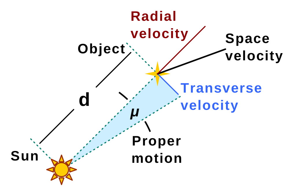
Consider an object $O$ that is a source of light. Let $S$ be a given frame of reference. Assume that $O$ has a radial velocity $v_{r}$ relative to $S$. Let $S^{\prime}$ be the rest frame of $O$. We now examine how the radial velocity $v_{r}$ affects the wavelength $\lambda$ of the light emitted by $O$, as measured in $S$. Let $\lambda_{0}$ be the wavelength of the light as measured in $S^{\prime}$. An observer in $S$ measures $\Delta t$, the time between the arrivals of two successive wave crests. Let $\Delta t^{\prime}$ be the same interval as measured in $S^{\prime}$. For now we ignore time dilation. The interval between emissions is then $\Delta t^{\prime}$ in both frames. During that interval the source recedes by $v_{r}\,\Delta t^{\prime}$, so the second crest must travel that much farther to reach the observer. Light covers the extra distance in a time $v_{r}\,\Delta t^{\prime}$. The observed interval is therefore \[ \Delta t = \Delta t^{\prime} + v_{r}\,\Delta t^{\prime} = \Delta t^{\prime}(1 + v_{r}) \] The wavelength of the light is proportional to the interval between crests. Therefore \[ \frac{\lambda}{\lambda_{0}} = \frac{\Delta t}{\Delta t^{\prime}} = 1 + v_{r} \] This derivation does not take into account the relativistic effects of time dilation and length contraction. In other words, the derivation is based on the model of Newtonian mechanics. The equation above is the classical Doppler formula. The classical Doppler formula is valid only when the radial velocity $v_{r}$ is much smaller than the speed of light. When the radial velocity $v_{r}$ is comparable to the speed of light, we need to take into account the relativistic effects of time dilation and length contraction.
We now repeat the derivation while taking relativistic effects into account. Consider the same object $O$ receding from an observer in frame $S$ at radial velocity $v_{r}$. Let $S^{\prime}$ be $O$'s rest frame. Let $\Delta t^{\prime}$ be the period between successive crests in $S^{\prime}$. The source's clock runs slow in $S$. The interval between the two emissions in $S$ is therefore $\gamma\,\Delta t^{\prime}$, where $\gamma = 1/\sqrt{1 - v_{r}^2}$. During that interval the source recedes by $v_{r}\,\gamma\,\Delta t^{\prime}$, so the second crest must travel that much farther. Light covers the extra distance in a time $v_{r}\,\gamma\,\Delta t^{\prime}$. The observed interval is therefore \[ \Delta t = \gamma\,\Delta t^{\prime} + v_{r}\,\gamma\,\Delta t^{\prime} = \gamma\,\Delta t^{\prime}(1 + v_{r}) \] As in the classical derivation, $\frac{\lambda}{\lambda_{0}} = \frac{\Delta t}{\Delta t^{\prime}}$. Therefore, \[ \frac{\lambda}{\lambda_{0}} = \gamma(1 + v_{r}) = \frac{1 + v_{r}}{\sqrt{1 - v_{r}^2}} = \sqrt{\frac{1 + v_{r}}{1 - v_{r}}} \] The equation above is the relativistic Doppler formula. Its right-hand side is the k-factor $k$ from equation \eqref{eq:k-factor-velocity}. This is the same $k$ we derived using k-calculus.
Now suppose $O$ moves transversely, perpendicular to the line of sight. Its radial velocity is then zero. No crest has to travel any farther than the one before it, so the light-travel stretching disappears. Only time dilation remains. The observed interval is the time-dilated emission interval, $\Delta t = \gamma\,\Delta t^{\prime}$. The shift is therefore \[ \frac{\lambda}{\lambda_{0}} = \frac{\Delta t}{\Delta t^{\prime}} = \frac{\gamma\,\Delta t^{\prime}}{\Delta t^{\prime}} = \gamma = \frac{1}{\sqrt{1 - v_{t}^2}} \] where $v_{t}$ is the transverse speed of $O$. The shift above is the transverse Doppler effect. Note that the transverse Doppler effect has no counterpart in the classical Doppler formula. It is a pure consequence of time dilation.
Mass and Energy
The Newtonian Mechanics section defined the linear momentum of a body as $p = m v$ in equation \eqref{eq:linear-momentum}. We showed that the total linear momentum of an isolated system stays constant. We now ask whether the same conservation law survives in special relativity. The Newtonian momentum measures the rate of change of an object's position with respect to the coordinate time $t$. Different observers assign different coordinate times to the same pair of events. If we assume the Newtonian momentum is conserved in one inertial frame, the velocity composition law \eqref{eq:velocity-composition} shows that it is not conserved in another. We repair the definition by measuring the rate of change of position against a time that every observer agrees on.
Recall that proper time $\tau$ from equation \eqref{eq:proper-time} is the time a moving clock records along its own worldline. Every observer computes the same proper time for a given stretch of worldline. Consider a particle of mass $m$ moving with velocity $v$ in an inertial frame. We define the particle's relativistic momentum to be the particle's mass multiplied by the rate of change of its position with respect to its proper time, \[ p = m \frac{\mathrm{d}x}{\mathrm{d}\tau} \] Over an infinitesimal step the proper time advances by $\mathrm{d}\tau = \sqrt{1 - v^2}\,\mathrm{d}t$, from equation \eqref{eq:proper-time}. The chain rule then gives \begin{equation}\label{eq:relativistic-momentum} p = m \frac{\mathrm{d}x}{\mathrm{d}t}\frac{\mathrm{d}t}{\mathrm{d}\tau} = m v (\frac{1}{\mathrm{d}\tau/\mathrm{d}t}) = \frac{m v}{\sqrt{1 - v^2}} = \gamma m v \end{equation} where $\gamma = 1/\sqrt{1 - v^2}$ and $v = \mathrm{d}x/\mathrm{d}t$ is the particle's velocity. Note that the mass $m$ keeps the same value in every frame. Also note that when $v$ is much less than $c = 1$, $\gamma$ is close to $1$. The relativistic momentum then reduces to the Newtonian momentum $m v$ of equation \eqref{eq:linear-momentum}. As $v$ approaches the speed of light, $\gamma$ grows without bound. The momentum $\gamma m v$ of a particle with nonzero mass therefore grows without bound as well. A particle with nonzero mass cannot reach the speed of light, since reaching it would require infinite momentum.
To define the relativistic momentum we differentiated the position $x$ with respect to the proper time and multiplied by the mass. Differentiating the time $t$ with respect to the proper time and multiplying by the mass gives a second quantity, $m\,\mathrm{d}t/\mathrm{d}\tau$. We define the total energy of the particle to be \begin{equation}\label{eq:relativistic-energy} E = m \frac{\mathrm{d}t}{\mathrm{d}\tau} = \frac{m}{\sqrt{1 - v^2}} = \gamma m \end{equation} To see why the name fits, we expand $\gamma$ for a small velocity. A Taylor expansion gives $\gamma \approx 1 + \tfrac{1}{2} v^2$. Substituting into equation \eqref{eq:relativistic-energy} gives \[ E \approx m + \tfrac{1}{2} m v^2 \] The second term is the Newtonian kinetic energy of the particle. The first term is a new quantity that is present even when the particle is at rest. We define the rest energy to be the energy $E = m$ of a particle at rest. Restoring the factors of the speed of light gives the familiar form $E = m c^2$. Mass is therefore a form of energy. We define the kinetic energy to be the energy above the rest energy, $K = E - m = (\gamma - 1) m$.
The energy and the momentum each depend on the frame. A different frame measures a different velocity for the particle, and therefore a different energy and a different momentum. However, there is a combination of the energy and the momentum that does not change from frame to frame. We compute $E^2 - p^2$ in a frame where the particle moves with velocity $v$, using $E = \gamma m$ from equation \eqref{eq:relativistic-energy} and $p = \gamma m v$ from equation \eqref{eq:relativistic-momentum}, \begin{equation}\label{eq:energy-momentum-relation} E^2 - p^2 = \gamma^2 m^2 - \gamma^2 m^2 v^2 = \gamma^2 m^2 (1 - v^2) = m^2 \end{equation} The result is $m^2$. The same computation holds in any frame, with that frame's velocity for the particle. The mass is the same in every frame. The combination $E^2 - p^2$ therefore equals $m^2$ in every inertial frame, in the same way the spacetime interval from equation \eqref{eq:interval} satisfies $s^{\prime 2} = s^2$ for any two inertial frames.
The relation $E^2 - p^2 = m^2$ ties the energy and the momentum, which change from frame to frame, to the mass, which does not. The pair $(E, p)$ and the pair $(t, x)$ share the same invariant structure. We call $(E, p)$ the energy-momentum four-vector, the counterpart of the coordinates $(t, x)$. Restoring the factors of the speed of light gives $E^2 - (p c)^2 = (m c^2)^2$.
Everything above describes an object with nonzero mass. Light needs a separate treatment. The definitions of the momentum and the energy in equations \eqref{eq:relativistic-momentum} and \eqref{eq:relativistic-energy} both measure a rate of change with respect to the proper time. Two events on the path of a light ray have a null spacetime interval. A clock carried along with the light therefore records no proper time between the two events. However, light still carries energy and momentum. For example, sunlight warms whatever it falls on. Light also pushes on whatever absorbs it. We now find the relation between the energy and the momentum of light.
Dividing equation \eqref{eq:relativistic-momentum} by equation \eqref{eq:relativistic-energy} gives \[ \frac{p}{E} = \frac{\gamma m v}{\gamma m} = v \] for an object with nonzero mass. The ratio of the momentum to the energy is the object's velocity. The energy and the momentum each grow without bound as the velocity approaches the speed of light. However, their ratio stays equal to the velocity and approaches $1$. Light travels at... well... the speed of light. We therefore assign light an energy and a momentum of equal size, \begin{equation}\label{eq:light-energy-momentum} E = p \end{equation} Restoring the factors of the speed of light gives $E = p c$.
Equation \eqref{eq:light-energy-momentum} gives $E^2 - p^2 = 0$. Comparing with equation \eqref{eq:energy-momentum-relation}, the mass of light is zero. We define an object to be massless when its mass is zero. Light is massless. We can also deduce that any massless object travels at the speed of light. The combination $E^2 - p^2$ vanishes for light in the same way the spacetime interval $s^2$ vanishes between two events on a light ray. We will use the energy and the momentum of light later, when we study how gravity bends light and shifts its wavelength.
Other treatments of relativity often describe light as a stream of particles and call each particle a photon. The particle description of light comes from quantum mechanics, which we do not develop in this book. A photon carries an energy and a momentum that satisfy equation \eqref{eq:light-energy-momentum}. Nothing we do with light later in the book needs more than the relation $E = p$.
Manifolds and Tensors
The coordinate systems we have used so far in our discussion of special relativity make the assumption that we can assign a unique set of four real numbers to every event in spacetime. Specifically, the coordinates $(t, x, y, z)$ of an event are the time and the three spatial coordinates of the event in a given inertial frame. The assumption holds throughout special relativity, where one inertial frame reaches every event. The assumption fails for other sets of points. As an example, one coordinate system does not suffice for the surface of a sphere. We give the reason below.
General relativity needs a more general framework for two separate reasons. First, spacetime can have a shape that no single coordinate system covers, in the same way the surface of a sphere does. Second, general relativity singles out no preferred coordinate system, while special relativity singles out the inertial frames. We develop both points later in the book. Hence we need two new mathematical structures. A manifold is a set of points that we cover with coordinate systems that each reach only a part of the set. A tensor is an object whose components in one coordinate system determine its components in every other coordinate system through a fixed rule. In this part we introduce manifolds first and tensors afterwards.
Manifolds
Consider the surface of a sphere. Latitude and longitude nearly assign a unique pair of numbers to each point of the surface. The assignment fails at the two poles, where every value of longitude names the same point. Away from the poles a small patch of a sphere resembles a small patch of a plane. A plane extends forever, however. A sphere has finite extent. A sphere and a plane therefore resemble each other near a point while differing as a whole.
Definition. A local property of a set of points is a property that depends only on a small patch around a point. A global property of a set of points is a property of the set taken in its entirety.
Example. A sphere resembling a plane in a small patch around a point is a local property. A plane extending forever is a global property.
We write $\mathbb{R}^n$ for the set of ordered $n$-tuples of real numbers. We write $x \in W$ when $x$ is an element of a set $W$. We write $V \subseteq W$ when every element of a set $V$ is an element of $W$. The notation $\{x \in W : \dots\}$ stands for the set of elements $x$ of $W$ that satisfy the condition after the colon. We write $W \setminus V = \{x \in W : x \text{ is not an element of } V\}$ for the set $W$ with the elements of $V$ removed. We write $V \cup W$ and $V \cap W$ for the union and the intersection of $V$ and $W$, and $\emptyset$ for the empty set, the set with no elements. We want a precise definition of a set of points that looks like $\mathbb{R}^n$ near each of its points. One notion from the geometry of $\mathbb{R}^n$ comes first. The Euclidean distance between two points $x$ and $y$ of $\mathbb{R}^n$ is \[ |x - y| = \sqrt{(x^1 - y^1)^2 + \dots + (x^n - y^n)^2} \] where $x^{i}$ and $y^{i}$ are the $i$-th components of $x$ and $y$ respectively.
Definition. The open ball of radius $r \gt 0$ about a point $x \in \mathbb{R}^n$ is the set \[ B_r(x) = \{y \in \mathbb{R}^n : |y - x| \lt r\} \]
Definition. We call $V \subseteq \mathbb{R}^n$ an open set (also called an open subset) when every point $v \in V$ has an open ball $B_r(v) \subseteq V$ for some $r \gt 0$.
Example. Let $Q$ be the square without its edges, \[ Q = \{(x, y) \in \mathbb{R}^2 : 0 \lt x \lt 1 \text{ and } 0 \lt y \lt 1\} \] We show that $Q$ is an open set. We therefore need, for each point $q \in Q$, a radius $r \gt 0$ with $B_r(q) \subseteq Q$. Let $q = (a, b) \in Q$. The distances from $q$ to the four edges $x = 0$, $x = 1$, $y = 0$ and $y = 1$ are $a$, $1 - a$, $b$ and $1 - b$. All four distances are positive, since $q \in Q$. We take the radius to be the distance from $q$ to the nearest edge, \[ r = \min(a, 1 - a, b, 1 - b) \] Let $(u, v) \in B_r(q)$. The number $\sqrt{(u - a)^2}$ equals $|u - a|$. Adding the non-negative term $(v - b)^2$ under the square root can only increase the value. The definition of $B_r(q)$ bounds the distance from $(u, v)$ to $q$ by $r$. Together the three facts give \[ |u - a| \le \sqrt{(u - a)^2 + (v - b)^2} \lt r \] The bound $|u - a| \lt r$ means $a - r \lt u \lt a + r$. The choice of $r$ gives $r \le a$ and $r \le 1 - a$, which means $a - r \ge 0$ and $a + r \le 1$. The first coordinate of $(u, v)$ therefore satisfies \[ 0 \le a - r \lt u \lt a + r \le 1 \] The same steps with $b$ in place of $a$ give $0 \lt v \lt 1$. The point $(u, v)$ therefore lies in $Q$. The point $(u, v)$ was any point of $B_r(q)$. The inclusion $B_r(q) \subseteq Q$ therefore holds. The square $Q$ is therefore an open set.
Example. Let $\bar{Q}$ be the square with its edges included, \[ \bar{Q} = \{(x, y) \in \mathbb{R}^2 : 0 \le x \le 1 \text{ and } 0 \le y \le 1\} \] We show that $\bar{Q}$ is not an open set. An open set $V$ has a radius $r \gt 0$ with $B_r(v) \subseteq V$ at every point $v \in V$. One point $q \in \bar{Q}$ with $B_r(q) \subseteq \bar{Q}$ for no $r \gt 0$ is therefore enough. We take the point $q = (0, 1/2)$ on the left edge. We show that $B_r(q) \subseteq \bar{Q}$ fails for every $r \gt 0$.
Let $r \gt 0$. The point $(-r/2, 1/2)$ lies at distance $r/2 \lt r$ from $q$. The point $(-r/2, 1/2)$ therefore lies in $B_r(q)$. The first coordinate $-r/2$ of the point is negative. The point $(-r/2, 1/2)$ therefore lies outside $\bar{Q}$. The inclusion $B_r(q) \subseteq \bar{Q}$ therefore fails. The number $r$ was any positive number. No $r \gt 0$ therefore satisfies $B_r(q) \subseteq \bar{Q}$. The square $\bar{Q}$ is therefore not an open set.
We need open sets for one reason. A partial derivative at a point uses the values of a function at nearby points in every direction. A function therefore needs room around a point before we can differentiate the function there. An open set contains an open ball about each of its points. A function whose domain is an open set therefore has room around every point of its domain.
Definition. Let $V \subseteq \mathbb{R}^n$ be an open set. A function $f : V \to \mathbb{R}^m$ is smooth when the partial derivatives of $f$ of every order exist and are continuous on $V$.
Let $M$ be a set. We call the elements of $M$ points. A point of $M$ has no structure of its own. We build every structure on $M$ from charts. A chart assigns numbers to points by a function. We write $f : A \to B$ for a function $f$ that takes each element of a set $A$ to an element of a set $B$. The set $A$ is the domain of $f$. The set $B$ is the codomain of $f$.
Definition. The identity function on a set $A$ is the function $A \to A$ that sends every $a \in A$ to $a$.
Definition. Let $f : A \to B$ be a function.
- The function $f$ is one-to-one, or injective, when $f(a_1) = f(a_2) \implies a_1 = a_2$ for every pair of elements $a_1$ and $a_2$ of $A$.
- The function $f$ is surjective, or maps $A$ onto $B$, when every $b \in B$ equals $f(a)$ for some $a \in A$.
- The function $f$ is a bijection when $f$ is both injective and surjective.
Definition. A coordinate chart on a set $M$ is a pair $(U, \psi)$, where $U \subseteq M$ and $\psi : U \to \mathbb{R}^n$ is an injective function whose image $\psi(U) = \{\psi(p) : p \in U\}$ is an open subset of $\mathbb{R}^n$. The subset $U$ is the domain of the chart. The function $\psi$ is the chart function. The coordinates of a point $p \in U$ in the chart are the $n$ numbers \[ \psi(p) = (x^1, x^2, \dots, x^n) \]
The image $\psi(U)$ is the set $\{\psi(p) : p \in U\}$. Every element of $\psi(U)$ therefore equals $\psi(p)$ for some $p \in U$. The function $\psi : U \to \psi(U)$, which has the same rule as the chart function and the smaller codomain $\psi(U)$, is therefore surjective. The function $\psi : U \to \psi(U)$ is also injective, since the implication $\psi(p) = \psi(q) \implies p = q$ does not depend on the codomain. The function $\psi : U \to \psi(U)$ is therefore a bijection. Each $n$-tuple of $\psi(U)$ equals $\psi(p)$ for exactly one point $p \in U$. The bijection therefore has an inverse function $\psi^{-1} : \psi(U) \to U$ with \[ \psi^{-1}(\psi(p)) = p \quad \text{for every } p \in U \] We use $\psi^{-1}$ when we compare two charts. We defined a coordinate system in the Preliminaries section as an origin together with a set of axes. A coordinate chart generalizes the notion. A chart needs no origin and no axes. A chart needs only to assign $n$ numbers to each point of its domain. Other treatments of manifolds call a coordinate chart a coordinate patch.
A function $f : A \to B$ assigns exactly one element of $B$ to each element of $A$. An assignment of numbers to points need not do so.
Definition. A rule on a set $A$ is an assignment of $n$-tuples to the points of $A$ that may give a point one $n$-tuple, several, or none.
Every function $A \to \mathbb{R}^n$ is therefore a rule on $A$. A rule on $A$ gives coordinates to the points of $A$ only when each point receives exactly one $n$-tuple and no two points receive the same $n$-tuple.
Definition. Let $\psi$ be a rule on a set $A$. The rule $\psi$ is degenerate at a point $p \in A$ when at least one of two conditions holds.
- The rule $\psi$ assigns more than one $n$-tuple, or no $n$-tuple, to $p$.
- The rule $\psi$ assigns to $p$ an $n$-tuple that $\psi$ also assigns to some point $q \in A$ with $q \ne p$.
The rule $\psi$ is non-degenerate when $\psi$ is degenerate at no point of $A$.
Let $\psi$ be a non-degenerate rule on $A$. Condition 1 holds at no point of $A$. The rule $\psi$ therefore assigns exactly one $n$-tuple to each point of $A$. The rule $\psi$ is therefore a function $\psi : A \to \mathbb{R}^n$. Condition 2 holds at no point of $A$ either. Two points $p, q \in A$ with $\psi(p) = \psi(q)$ are therefore the same point, which gives \[ \psi(p) = \psi(q) \implies p = q \] for every $p, q \in A$. A non-degenerate rule on $A$ is therefore an injective function $A \to \mathbb{R}^n$. Conversely, a function $\psi : A \to \mathbb{R}^n$ assigns exactly one $n$-tuple to each point of $A$. Condition 1 therefore holds at no point. An injective function also assigns distinct $n$-tuples to distinct points. Condition 2 therefore holds at no point either. A rule on $A$ is therefore non-degenerate exactly when the rule is an injective function $A \to \mathbb{R}^n$. The chart function $\psi$ of a coordinate chart $(U, \psi)$ is injective. A coordinate chart $(U, \psi)$ is therefore non-degenerate on $U$.
Example. Plane polar coordinates are a rule on $\mathbb{R}^2$. The rule assigns to a point $(x, y)$ every pair $(r, \theta)$ with $r \ge 0$ and $0 \le \theta \lt 2\pi$ that satisfies \[ (x, y) = (r\cos\theta, r\sin\theta) \] The origin satisfies the equation with $r = 0$ and every value of $\theta$. The rule therefore assigns more than one pair to the origin. Plane polar coordinates are therefore degenerate at the origin by condition 1. The rule assigns exactly one pair to every other point of the plane. Distinct points also receive distinct pairs. Plane polar coordinates are therefore non-degenerate on $\mathbb{R}^2 \setminus \{(0, 0)\}$. Restricting a rule to a smaller set in this way is a common way to avoid degeneracy. The domain of a chart is therefore often only part of a set.
A single chart need not reach every point of a set $M$. We therefore use several charts at once.
Definition. Let $I$ be a set of indices. An atlas on a set $M$ is a collection $\{(U_i, \psi_i) : i \in I\}$ of charts on $M$, one chart for each index $i \in I$, that meets two conditions.
- Every point of $M$ belongs to the domain $U_i$ of at least one chart.
- For every pair of charts $(U_i, \psi_i)$ and $(U_j, \psi_j)$ of the collection, both $\psi_i(U_i \cap U_j)$ and $\psi_j(U_i \cap U_j)$ are open subsets of $\mathbb{R}^n$.
The index set $I$ may be finite or infinite. An atlas on the sphere needs only the index set $I = \{1, 2\}$, as the sphere example later in this section shows. The first condition gives every point of $M$ coordinates in at least one chart of the atlas. The domains of two charts of an atlas may overlap. A point in the overlap $U_i \cap U_j$ then has one set of coordinates from each of the two charts.
Let $(U_i, \psi_i)$ and $(U_j, \psi_j)$ be charts of an atlas whose domains overlap. A point $p$ of the overlap has the coordinates $\psi_i(p)$ from the first chart and the coordinates $\psi_j(p)$ from the second.
Definition. The transition function from $(U_i, \psi_i)$ to $(U_j, \psi_j)$ is the function $\psi_j \circ \psi_i^{-1}$, which sends $\psi_i(p)$ to $\psi_j(p)$ for every point $p$ of $U_i \cap U_j$.
The transition function takes the coordinates in the first chart of the points of the overlap to their coordinates in the second chart, \[ \psi_j \circ \psi_i^{-1} : \psi_i(U_i \cap U_j) \to \psi_j(U_i \cap U_j) \] Condition 2 of makes the domain $\psi_i(U_i \cap U_j)$ of the transition function an open subset of $\mathbb{R}^n$. A partial derivative of a function at a point $x$ uses the values of the function at the points obtained by changing one coordinate of $x$ by a small amount of either sign. An open ball $B_r(x)$ in the domain contains every such point whose change is smaller than $r$. We defined a smooth function only on an open subset of $\mathbb{R}^n$ for that reason. therefore applies to the transition function $\psi_j \circ \psi_i^{-1}$.
Definition. Let $n$ be a positive integer and let $I$ be a set of indices. A manifold of dimension $n$ is a set $M$ together with an atlas $\{(U_i, \psi_i) : i \in I\}$ on $M$ that meets two conditions.
- Every chart of the atlas assigns exactly $n$ coordinates to each point of its domain, i.e., $\psi_i : U_i \to \mathbb{R}^n$ for every $i$.
- For every pair of charts $(U_i, \psi_i)$ and $(U_j, \psi_j)$ whose domains overlap, the transition function $\psi_j \circ \psi_i^{-1}$ is smooth.
The number $n$ is the dimension of the manifold.
A fuller name for a manifold is a smooth manifold. Every manifold in this book is smooth.
We write the coordinates of a chart as $x^a$, with the index $a$ running from $1$ to $n$. Lower case Latin indices run from $1$ to $n$ throughout the rest of the book. The index is a superscript. The position of an index has a meaning. We will meet quantities whose indices are subscripts. Quantities of the two kinds change differently under a change of chart. A superscript on a coordinate tells us which of the $n$ coordinates we mean. A superscript on a coordinate is never an exponent. The symbol $x^2$ denotes the second coordinate of a chart. The square of the second coordinate is $(x^2)^2$.
Let $(U_i, \psi_i)$ and $(U_j, \psi_j)$ be charts whose domains overlap. We write $\psi_i(p) = (x^1, \dots, x^n)$ and $\psi_j(p) = (x^{\prime 1}, \dots, x^{\prime n})$ for the coordinates of a point $p \in U_i \cap U_j$ in the two charts. The transition function $\psi_j \circ \psi_i^{-1}$ and the inverse transition function $\psi_i \circ \psi_j^{-1}$ give each coordinate of one chart as a function of the coordinates of the other, \[ x^{\prime a} = x^{\prime a}(x^1, \dots, x^n) \qquad x^a = x^a(x^{\prime 1}, \dots, x^{\prime n}) \] Condition 2 of makes both transition functions smooth. The partial derivatives of these $2n$ functions therefore exist. In the Changing Charts section the partial derivatives form two transformation matrices, and shows that the two matrices are inverses of each other.
Example. A sphere needs more than one chart. We do not prove this in this book but no chart whose chart function is continuous has the whole sphere as its domain. However, it is possible to build an atlas on the sphere with two charts. Let $S$ be the sphere \[ S = \{(x, y, z) \in \mathbb{R}^3 : x^2 + y^2 + z^2 = 1\} \] We call $p_{\mathrm{N}} = (0, 0, 1)$ the north pole and $p_{\mathrm{S}} = (0, 0, -1)$ the south pole. Both chart functions send a point of $S$ to a point $(X, Y, 0)$ of the plane $z = 0$. The coordinates of the point of $S$ are then $(X, Y) \in \mathbb{R}^2$. Let $U_1 = S \setminus \{p_{\mathrm{S}}\}$. Drawing the line from $p_{\mathrm{S}}$ through a point of $U_1$ and recording where the line meets the plane $z = 0$ gives \[ \psi_1(x, y, z) = \left(\frac{x}{1 + z},\ \frac{y}{1 + z}\right) \] Let $U_2 = S \setminus \{p_{\mathrm{N}}\}$. Drawing the line from $p_{\mathrm{N}}$ gives \[ \psi_2(x, y, z) = \left(\frac{x}{1 - z},\ \frac{y}{1 - z}\right) \] The denominator $1 + z$ equals $0$ only at $p_{\mathrm{S}}$, which does not lie in $U_1$. The denominator $1 - z$ equals $0$ only at $p_{\mathrm{N}}$, which does not lie in $U_2$. Each function is therefore defined on the whole of its domain. The only point of $S$ outside $U_1$ is $p_{\mathrm{S}}$. The south pole satisfies $p_{\mathrm{S}} \in U_2$. The two domains therefore satisfy $U_1 \cup U_2 = S$. The overlap is $U_1 \cap U_2 = S \setminus \{p_{\mathrm{N}}, p_{\mathrm{S}}\}$. The function $\psi_1$ sends $p_{\mathrm{N}}$ to the origin. The image of the overlap is therefore \[ \psi_1(U_1 \cap U_2) = \mathbb{R}^2 \setminus \{(0, 0)\} \] The same holds for $\psi_2$, which sends $p_{\mathrm{S}}$ to the origin. Let $u \in \mathbb{R}^2 \setminus \{(0, 0)\}$. The distance from $u$ to the origin is $|u| \gt 0$. The open ball $B_{|u|}(u)$ therefore does not contain the origin, which gives $B_{|u|}(u) \subseteq \mathbb{R}^2 \setminus \{(0, 0)\}$. The set $\mathbb{R}^2 \setminus \{(0, 0)\}$ is therefore an open set. Both conditions of therefore hold.
We now compute the transition function from $(U_1, \psi_1)$ to $(U_2, \psi_2)$. Let $p = (x, y, z) \in U_1 \cap U_2$ and let $u = \psi_1(p)$. Every point of $S$ satisfies $x^2 + y^2 = 1 - z^2$. The squared length of $u$ is therefore \[ |u|^2 = \frac{x^2 + y^2}{(1 + z)^2} = \frac{1 - z^2}{(1 + z)^2} = \frac{1 - z}{1 + z} \] Multiplying $u$ by $1 / |u|^2 = (1 + z) / (1 - z)$ gives \[ \frac{u}{|u|^2} = \left(\frac{x}{1 - z},\ \frac{y}{1 - z}\right) = \psi_2(p) \] The transition function $\psi_2 \circ \psi_1^{-1}$ therefore sends $u$ to $u / |u|^2$. The function $u \mapsto u / |u|^2$ has partial derivatives of every order at every point where $|u| \neq 0$. The origin does not lie in $\psi_1(U_1 \cap U_2)$. The transition function is therefore smooth. Swapping the roles of the two charts gives the same formula for the transition function in the other order. The set $S$ together with the two charts is therefore a manifold of dimension two.
Spacetime in general relativity is a manifold of dimension four. The definitions above already hold for a manifold of any dimension $n$. We keep the dimension general for the rest of this part, since the extra generality costs us nothing.
Subspaces of Another Kind
For the entirety of this section, let $M$ be a manifold of dimension $n$ with atlas $\{(U_i, \psi_i) : i \in I\}$.
Definition. A curve in $M$ is a function $\gamma : K \to M$, where $K = (\alpha, \beta)$ is an open interval in $\mathbb{R}$.
We call the variable $u \in K$ the parameter of the curve $\gamma$ and the set $\gamma(K) = \{\gamma(u) : u \in K\}$ the image of the curve $\gamma$. Two different curves can have the same image, as the unit circle example later in this section shows. The image $\gamma(K)$ therefore does not determine the curve $\gamma$.
Definition. Let $\gamma : K \to M$ be a curve and let $(U_i, \psi_i)$ be a chart. Let $J_i = \{u \in K : \gamma(u) \in U_i\}$ be the set of parameter values at which the curve is in $U_i$. The coordinate representation of the curve $\gamma$ in the chart $(U_i, \psi_i)$ is the $n$ functions $x^a : J_i \to \mathbb{R}$ given by \begin{equation}\label{eq:curve} \psi_i(\gamma(u)) = (x^1(u), x^2(u), \dots, x^n(u)), \qquad u \in J_i \end{equation}
Definition. A curve $\gamma : K \to M$ is smooth when every chart $(U_i, \psi_i)$ of the atlas satisfies two conditions.
- The set $J_i = \{u \in K : \gamma(u) \in U_i\}$ is an open subset of $\mathbb{R}$.
- Each function $x^a : J_i \to \mathbb{R}$ of the coordinate representation of the curve $\gamma$ in the chart $(U_i, \psi_i)$ is smooth.
Condition 1 is necessary for condition 2 since we defined a smooth function only on an open subset. Every curve in this book is smooth.
Let $(U_i, \psi_i)$ and $(U_j, \psi_j)$ be two charts of the atlas $\{(U_i, \psi_i) : i \in I\}$ of the manifold $M$. Let $x^a : J_i \to \mathbb{R}$ and $x^{\prime a} : J_j \to \mathbb{R}$ be the coordinate representations of the curve $\gamma$ in the two charts. For every $u \in J_i \cap J_j$, the point $\gamma(u)$ belongs to $U_i \cap U_j$ by the definitions of $J_i$ and $J_j$ in . Hence the chart function $\psi_i$ and the inverse chart function $\psi_i^{-1}$ satisfy $\psi_i^{-1}(\psi_i(\gamma(u))) = \gamma(u)$ for every $u \in J_i \cap J_j$. From this, we can derive \[ \begin{aligned} \left(x^{\prime 1}(u), \dots, x^{\prime n}(u)\right) &= \psi_j(\gamma(u)) \\ &= \psi_j\left(\psi_i^{-1}(\psi_i(\gamma(u)))\right) \\ &= (\psi_j \circ \psi_i^{-1})\left(x^1(u), \dots, x^n(u)\right) \end{aligned} \] Recall that the transition function $\psi_j \circ \psi_i^{-1}$ gives each coordinate $x^{\prime a}$ of a point $p \in U_i \cap U_j$ in the chart $(U_j, \psi_j)$ as a function $x^{\prime a}(x^1, \dots, x^n)$ of the coordinates $x^1, \dots, x^n$ of the same point $p$ in the chart $(U_i, \psi_i)$. Component $a$ of the last line is therefore \begin{equation}\label{eq:curve-chart-change} x^{\prime a}(u) = x^{\prime a}\left(x^1(u), \dots, x^n(u)\right), \qquad u \in J_i \cap J_j \end{equation} Condition 2 of makes the functions $x^{\prime a}(x^1, \dots, x^n)$ smooth. A composition of smooth functions is smooth. Condition 2 in the chart $(U_i, \psi_i)$ therefore implies condition 2 in the chart $(U_j, \psi_j)$ on $J_i \cap J_j$. To check condition 2 for the curve $\gamma$ near a point $p$ of $M$, we therefore need not check every chart whose domain contains $p$. Any one such chart is enough, since condition 2 in that chart implies condition 2 near $p$ in all the others.
Example. The set $\mathbb{R}^n$ is a manifold of dimension $n$ with an atlas of one chart $(\mathbb{R}^n, \psi_1)$, whose chart function $\psi_1$ is the identity function on $\mathbb{R}^n$. The one transition function $\psi_1 \circ \psi_1^{-1}$ is the identity function, which is smooth. We take the dimension of the manifold to be $n = 2$ and the open interval $K$ to be all of $\mathbb{R}$. The two curves \[ \gamma_1(u) = (\cos u, \sin u) \qquad \gamma_2(u) = (\cos 2u, \sin 2u) \] both have the unit circle as their image. The two curves are different functions, since $\gamma_1(\pi) = (-1, 0)$ and $\gamma_2(\pi) = (1, 0)$. Each curve reaches every point of the unit circle at infinitely many parameter values, since $\cos$ and $\sin$ repeat after $2\pi$. The chart function $\psi_1$ is the identity function. The coordinate representation of $\gamma_1$ is therefore $x^1(u) = \cos u$ and $x^2(u) = \sin u$, which are smooth on $J_1 = \mathbb{R}$.
We have met curves in the physical setting already. A worldline is a curve in spacetime.
A curve has one parameter. A function with more parameters gives a set of points of higher dimension.
Definition. Let $m$ be an integer with $1 \le m \le n$ and let $D \subseteq \mathbb{R}^m$ be an open set. A subspace of $M$ of dimension $m$ is a function $\chi : D \to M$. Three special cases have names of their own.
- A subspace of dimension $1$ with $D$ an open interval is a curve.
- A subspace of dimension $2$ is a surface.
- A subspace of dimension $n - 1$ is a hypersurface.
The word subspace here has nothing to do with the linear algebra notion of the same name.
Definition. Let $\chi : D \to M$ be a subspace of dimension $m$ and let $(U_i, \psi_i)$ be a chart. Let $D_i = \{u \in D : \chi(u) \in U_i\}$. We write a point of $D_i$ as $u = (u^1, \dots, u^m)$. The parametric representation of the subspace $\chi$ in the chart $(U_i, \psi_i)$ is the $n$ functions $x^a : D_i \to \mathbb{R}$ given by $\psi_i(\chi(u)) = (x^1(u), \dots, x^n(u))$, which we write as \begin{equation}\label{eq:subspace} x^a = x^a(u^1, u^2, \dots, u^m), \qquad a = 1, 2, \dots, n \end{equation}
The parametric representation of a curve is its coordinate representation. A subspace $\chi$ is smooth when every chart satisfies the two conditions of , with $D_i$ in place of $J_i$ and $\mathbb{R}^m$ in place of $\mathbb{R}$. Every subspace in this book is smooth.
The parametric representation gives the coordinates of the points of a subspace as functions of the parameters. A set of points can also be given by equations on the coordinates.
Definition. Let $\chi : D \to M$ be a subspace of dimension $m$, let $(U_i, \psi_i)$ be a chart whose domain $U_i$ contains the image $\chi(D)$, and let $V \subseteq \psi_i(U_i)$ be an open set. We write a point of $V$ as $x = (x^1, \dots, x^n)$. Functions $f^1, \dots, f^{\,n-m} : V \to \mathbb{R}$ form a constraint representation of the subspace $\chi$ in $V$ when the coordinates of the points of $\chi(D)$ are the solutions in $V$ of the $n - m$ equations, \begin{equation}\label{eq:subspace-constraints} \psi_i(\chi(D)) = \{x \in V : f^1(x) = \dots = f^{\,n-m}(x) = 0\} \end{equation}
A hypersurface has dimension $m = n - 1$, which gives $n - m = 1$. A constraint representation of a hypersurface is therefore a single equation \begin{equation}\label{eq:hypersurface-constraint} f(x^1, x^2, \dots, x^n) = 0 \end{equation}
Example. The sphere $S$ of the Manifolds section is a surface in the manifold $M = \mathbb{R}^3$. We use the atlas $\{(\mathbb{R}^3, \psi_1)\}$ of one chart, whose chart function $\psi_1$ is the identity function. The coordinates of a point $p \in M$ are therefore $\psi_1(p) = p = (x^1, x^2, x^3)$. We look at the parametric representation and the constraint representation of $S$.
The parametric representation of $S$ is \[ x^1 = \sin u^1 \cos u^2, \qquad x^2 = \sin u^1 \sin u^2, \qquad x^3 = \cos u^1 \] Each choice of the two parameters $u^1$ and $u^2$ gives a point of $S$. The parameters $u^1 = \pi/2$ and $u^2 = 0$ give the point $(1, 0, 0)$.
The constraint representation of $S$ is the single equation \[ (x^1)^2 + (x^2)^2 + (x^3)^2 - 1 = 0 \] which has the form \eqref{eq:hypersurface-constraint}. A point belongs to $S$ when its coordinates satisfy the equation. The point $(0, 0, 1)$ satisfies the equation and belongs to $S$. The point $(1, 1, 0)$ gives $1 + 1 + 0 - 1 = 1$ and does not belong to $S$.
The parametric representation produces the points of $S$. The constraint representation tests whether a given point belongs to $S$.
Changing Charts
For the entirety of this section, let $(U_i, \psi_i)$ and $(U_j, \psi_j)$ be two charts of the atlas $\{(U_i, \psi_i) : i \in I\}$ of the manifold $M$ with $U_i \cap U_j \neq \emptyset$. A point $p \in U_i \cap U_j$ has the coordinates $\psi_i(p) = (x^1, \dots, x^n)$ in the chart $(U_i, \psi_i)$ and the coordinates $\psi_j(p) = (x^{\prime 1}, \dots, x^{\prime n})$ in the chart $(U_j, \psi_j)$.
Definition. The coordinate transformation from the chart $(U_i, \psi_i)$ to the chart $(U_j, \psi_j)$ is the $n$ functions \begin{equation}\label{eq:coordinate-change} x^{\prime a} = x^{\prime a}(x^1, x^2, \dots, x^n), \qquad a = 1, 2, \dots, n \end{equation} that make up the transition function $\psi_j \circ \psi_i^{-1}$. The inverse coordinate transformation is the $n$ functions $x^a = x^a(x^{\prime 1}, \dots, x^{\prime n})$ that make up the transition function $\psi_i \circ \psi_j^{-1}$.
A coordinate transformation does not move the point $p$. The two charts assign different coordinates to the same point $p$. The coordinate transformation converts one set of coordinates into the other. The Lorentz transformation \eqref{eq:lorentz-standard} of the Special Relativity chapter is a coordinate transformation. It converts the coordinates of an event in one inertial frame into the coordinates of the same event in another inertial frame.
Definition. The coordinate transformation \eqref{eq:coordinate-change} from the chart $(U_i, \psi_i)$ to the chart $(U_j, \psi_j)$ comes with three quantities.
- The transformation matrix $\Lambda$ is the $n \times n$ matrix with the entry $\Lambda^a_b = \partial x^{\prime a} / \partial x^b$ in row $a$ and column $b$.
- The transformation matrix $N$ of the inverse coordinate transformation, from the chart $(U_j, \psi_j)$ to the chart $(U_i, \psi_i)$, is the $n \times n$ matrix with the entry $N^a_b = \partial x^a / \partial x^{\prime b}$ in row $a$ and column $b$.
- The Jacobian of the coordinate transformation is the determinant $J = \det \Lambda$.
Each entry $\Lambda^a_b$ is a function of the coordinates $x^1, \dots, x^n$. The transformation matrix $\Lambda$ therefore changes in general from one point of $U_i \cap U_j$ to another. The transformation matrix $N$ changes in the same way.
Example. We take the manifold $M = \mathbb{R}^2$ with the coordinates $(t, x)$ in one chart and the coordinates $(t^{\prime}, x^{\prime})$ in a second chart, related by the Lorentz boost $B_v$. Multiplying out the Lorentz transformation \eqref{eq:lorentz-standard} gives the coordinate transformation \[ t^{\prime} = \gamma t - \gamma v x \qquad x^{\prime} = -\gamma v t + \gamma x \] The numbers $\gamma$ and $v$ are constants. The transformation matrix is therefore \[ \Lambda = \begin{pmatrix} \dfrac{\partial t^{\prime}}{\partial t} & \dfrac{\partial t^{\prime}}{\partial x} \\[1.2ex] \dfrac{\partial x^{\prime}}{\partial t} & \dfrac{\partial x^{\prime}}{\partial x} \end{pmatrix} = \begin{pmatrix} \gamma & -\gamma v \\ -\gamma v & \gamma \end{pmatrix} = B_v \] The entries of $\Lambda$ do not depend on $t$ or $x$. The transformation matrix of a Lorentz boost is therefore the same at every point. The Jacobian is \[ J = \gamma^2 - \gamma^2 v^2 = \gamma^2 (1 - v^2) = 1 \] The last step uses $\gamma^2 = 1 / (1 - v^2)$.
Equation \eqref{eq:coordinate-change} makes each $x^{\prime a}$ a function of the $n$ coordinates $x^1, \dots, x^n$. The total differential of $x^{\prime a}$ is therefore \[ \mathrm{d}x^{\prime a} = \frac{\partial x^{\prime a}}{\partial x^1}\,\mathrm{d}x^1 + \dots + \frac{\partial x^{\prime a}}{\partial x^n}\,\mathrm{d}x^n = \sum_{b=1}^{n} \frac{\partial x^{\prime a}}{\partial x^b}\,\mathrm{d}x^b \] We meet sums of this shape throughout the rest of the book.
Definition. The Einstein summation convention sums an index that appears twice in a single product over the values $1$ to $n$ and leaves the summation sign out, \[ c_b \, v^b = \sum_{b=1}^{n} c_b \, v^b \] An index that appears once in each of two products added together is not summed, as in $c^a + v^a$.
The Einstein summation convention writes the total differential as \begin{equation}\label{eq:total-differential} \mathrm{d}x^{\prime a} = \frac{\partial x^{\prime a}}{\partial x^b}\,\mathrm{d}x^b \end{equation} In a manifold of dimension $3$, equation \eqref{eq:total-differential} with $a = 1$ stands for \[ \mathrm{d}x^{\prime 1} = \frac{\partial x^{\prime 1}}{\partial x^1}\,\mathrm{d}x^1 + \frac{\partial x^{\prime 1}}{\partial x^2}\,\mathrm{d}x^2 + \frac{\partial x^{\prime 1}}{\partial x^3}\,\mathrm{d}x^3 \]
Definition. In an equation written with the Einstein summation convention, an index that appears once in every term is a free index. An index that the convention sums is a dummy index. In the equation \[ w^a = \Lambda^a_b \, v^b \] the index $a$ is free and the index $b$ is a dummy index.
An equation holds for every value of its free indices. Equation \eqref{eq:total-differential}, whose free index is $a$, is therefore $n$ equations, one for each value of $a$. The expanded sum above contains no $b$. The letter of a dummy index therefore only marks which factors the convention sums. Replacing the letter by any other letter not already in use gives the same sum, \[ \frac{\partial x^{\prime a}}{\partial x^b}\,\mathrm{d}x^b = \frac{\partial x^{\prime a}}{\partial x^c}\, \mathrm{d}x^c \]
Definition. The Kronecker delta $\delta^a_b$ is the entry of the identity matrix $\mathbf{1}$ in row $a$ and column $b$, \begin{equation}\label{eq:kronecker-delta} \delta^a_b = \begin{cases} 1 & \text{if } a = b \\ 0 & \text{if } a \neq b \end{cases} \end{equation}
The coordinates $x^{\prime 1}, \dots, x^{\prime n}$ of the chart $(U_j, \psi_j)$ are independent variables. The partial derivative $\partial x^{\prime a} / \partial x^{\prime b}$ therefore equals $1$ when $a = b$ and $0$ when $a \neq b$. The same holds for the coordinates $x^1, \dots, x^n$ of the chart $(U_i, \psi_i)$, which gives \begin{equation}\label{eq:coordinate-derivative-delta} \frac{\partial x^{\prime a}}{\partial x^{\prime b}} = \delta^a_b \qquad \frac{\partial x^a}{\partial x^b} = \delta^a_b \end{equation}
Theorem. Let $(U_i, \psi_i)$ and $(U_j, \psi_j)$ be any two charts of a manifold $M$ with $U_i \cap U_j \neq \emptyset$. Let $\Lambda$ be the transformation matrix of the coordinate transformation from $(U_i, \psi_i)$ to $(U_j, \psi_j)$ and let $N$ be the transformation matrix of the inverse coordinate transformation, as in . At every point of $U_i \cap U_j$, the matrices $\Lambda$ and $N$ are inverses of each other, \begin{equation}\label{eq:matrix-inverse-index} \Lambda^a_b N^b_c = \delta^a_c \end{equation}
Proof. Let $p$ be any point of $U_i \cap U_j$. We write $x = \psi_i(p)$ and $x^{\prime} = \psi_j(p)$ for the coordinates of $p$ in the two charts. By , the coordinate transformation gives $x^{\prime}$ as the function $x^{\prime a}(x^1, \dots, x^n)$ of $x$. The inverse coordinate transformation gives $x$ as the function $x^b(x^{\prime 1}, \dots, x^{\prime n})$ of $x^{\prime}$. Substituting the second into the first gives \begin{equation}\label{eq:composite-coordinates} x^{\prime a} = x^{\prime a}\left(x^1(x^{\prime}), \dots, x^n(x^{\prime})\right) \end{equation} The point $p$ is any point of $U_i \cap U_j$. Equation \eqref{eq:composite-coordinates} therefore holds for every $x^{\prime}$ in the open set $\psi_j(U_i \cap U_j)$, which lets us differentiate both sides with respect to $x^{\prime c}$. For a function $f(x^1, \dots, x^n)$, the chain rule states that \begin{equation}\label{eq:chain-rule-n} \frac{\partial}{\partial x^{\prime c}}\Big( f\left(x^1(x^{\prime}), \dots, x^n(x^{\prime})\right) \Big) = \sum_{b=1}^{n} \frac{\partial f}{\partial x^b}\left(x^1(x^{\prime}), \dots, x^n(x^{\prime})\right) \frac{\partial x^b}{\partial x^{\prime c}}\left(x^{\prime}\right) \end{equation} Differentiating both sides of \eqref{eq:composite-coordinates} with respect to $x^{\prime c}$ gives \[ \begin{aligned} \delta^a_c &= \frac{\partial x^{\prime a}}{\partial x^{\prime c}} \\ &= \frac{\partial}{\partial x^{\prime c}}\Big( x^{\prime a}\left(x^1(x^{\prime}), \dots, x^n(x^{\prime})\right) \Big) \\ &= \sum_{b=1}^{n} \frac{\partial x^{\prime a}}{\partial x^b}\left(x^1(x^{\prime}), \dots, x^n(x^{\prime})\right) \frac{\partial x^b}{\partial x^{\prime c}}\left(x^{\prime}\right) \\ &= \sum_{b=1}^{n} \frac{\partial x^{\prime a}}{\partial x^b}(x) \, \frac{\partial x^b}{\partial x^{\prime c}} (x^{\prime}) \\ &= \frac{\partial x^{\prime a}}{\partial x^b}(x) \, \frac{\partial x^b}{\partial x^{\prime c}}(x^{\prime}) \\ &= \Lambda^a_b N^b_c \end{aligned} \] The first line is \eqref{eq:coordinate-derivative-delta}. The second line uses \eqref{eq:composite-coordinates}. The third line is \eqref{eq:chain-rule-n} with $f = x^{\prime a}$. The functions $x^b(x^{\prime})$ give the coordinates of $p$ in the chart $(U_i, \psi_i)$, which are $(x^1(x^{\prime}), \dots, x^n(x^{\prime})) = x$. The fourth line uses this equation. The fifth line writes the sum with the Einstein summation convention. The sixth line is at the point $p$. The result is \eqref{eq:matrix-inverse-index}, which states $\Lambda N = \mathbf{1}$ entry by entry. The matrix $N$ is therefore $\Lambda^{-1}$. $\blacksquare$
Corollary. For the charts of , the Jacobian $J = \det \Lambda$ is never zero. The inverse coordinate transformation has the Jacobian $\det N = 1 / J$.
Proof. The determinant of a product of matrices is the product of their determinants. then gives \[ J \det N = \det \Lambda \, \det N = \det(\Lambda N) = \det \mathbf{1} = 1 \] If $J$ were $0$, the left hand side would be $0 \cdot \det N = 0$, not $1$. The Jacobian $J$ is therefore not zero. Dividing by $J$ gives $\det N = 1 / J$. $\blacksquare$
For the Lorentz boost of the example above, $\Lambda = B_v$. By , $N = B_v^{-1} = B_{-v}$, the boost with the opposite velocity.
Contravariant Tensors
For the entirety of this section, let $(U_i, \psi_i)$ and $(U_j, \psi_j)$ be two charts of the atlas $\{(U_i, \psi_i) : i \in I\}$ of a manifold $M$ of dimension $n$, and let $p \in U_i \cap U_j$. The point $p$ has the coordinates $\psi_i(p) = (x^1, \dots, x^n)$ in the chart $(U_i, \psi_i)$ and the coordinates $\psi_j(p) = (x^{\prime 1}, \dots, x^{\prime n})$ in the chart $(U_j, \psi_j)$. We write \[ \mathcal{C}_p = \{(U_k, \psi_k) : k \in I \text{ and } p \in U_k\} \] for the set of charts of the atlas whose domains contain $p$. We also write \begin{equation}\label{eq:evaluation-at-p} \Lambda^a_b = \left[\frac{\partial x^{\prime a}}{\partial x^b}\right]_p = \frac{\partial x^{\prime a}}{\partial x^b}\left(\psi_i(p)\right) \end{equation} for the value of the function $\partial x^{\prime a} / \partial x^b$ at the coordinates $\psi_i(p)$ of $p$, the entry of the transformation matrix $\Lambda$ at the point $p$.
Consider a particle whose worldline is a curve $\gamma$ through the point $p$ of the manifold $M$. The chart $(U_i, \psi_i)$ describes the velocity of the particle at $p$ by $n$ numbers, the rates of change $\mathrm{d}x^a / \mathrm{d}u$ of its coordinates. The chart $(U_j, \psi_j)$ describes the same velocity by $n$ different numbers $\mathrm{d}x^{\prime a} / \mathrm{d}u$. No chart of $M$ is preferred. Neither list is therefore the velocity itself. We want a description of the velocity that does not depend on the chart. calls the $n$ numbers $\mathrm{d}x^a / \mathrm{d}u$ at $p$ the tangent vector in the chart $(U_i, \psi_i)$. We then find how these numbers change to the numbers $\mathrm{d}x^{\prime a} / \mathrm{d}u$ of the chart $(U_j, \psi_j)$.
Definition. Let $\gamma : K \to M$ be a smooth curve and let $u_0 \in K$ with $\gamma(u_0) = p$. Let $x^a(u)$ be the coordinate representation of the curve $\gamma$ in the chart $(U_i, \psi_i)$. The tangent vector to the curve $\gamma$ at the parameter value $u_0$ in the chart $(U_i, \psi_i)$ is the $n$ numbers \begin{equation}\label{eq:tangent-vector} T^a = \left[\frac{\mathrm{d}x^a}{\mathrm{d}u}\right]_{u_0} \end{equation}
The parameter value $u_0$ belongs to the set $J_i = \{u \in K : \gamma(u) \in U_i\}$ of , since $\gamma(u_0) = p \in U_i$. makes each function $x^a(u)$ smooth on the open set $J_i$. The derivatives $T^a$ therefore exist.
Let $T^{\prime a}$ be the tangent vector to the curve $\gamma$ at the parameter value $u_0$ in the chart $(U_j, \psi_j)$, where $x^{\prime a}(u)$ is the coordinate representation of $\gamma$ in that chart. Then \begin{equation}\label{eq:tangent-transformation} \begin{aligned} T^{\prime a} &= \left[\frac{\mathrm{d}x^{\prime a}}{\mathrm{d}u}\right]_{u_0} \\ &= \left[\frac{\mathrm{d}}{\mathrm{d}u}\, x^{\prime a}\left(x^1(u), \dots, x^n(u)\right)\right]_{u_0} \\ &= \left[\sum_{b=1}^{n} \frac{\partial x^{\prime a}}{\partial x^b}\left(x^1(u), \dots, x^n(u)\right) \frac{\mathrm{d}x^b}{\mathrm{d}u}\right]_{u_0} \\ &= \sum_{b=1}^{n} \frac{\partial x^{\prime a}}{\partial x^b}\left(x^1(u_0), \dots, x^n(u_0)\right) \left[\frac{\mathrm{d}x^b}{\mathrm{d}u}\right]_{u_0} \\ &= \sum_{b=1}^{n} \frac{\partial x^{\prime a}}{\partial x^b}\left(\psi_i(\gamma(u_0))\right) \left[\frac{\mathrm{d}x^b}{\mathrm{d}u}\right]_{u_0} \\ &= \sum_{b=1}^{n} \frac{\partial x^{\prime a}}{\partial x^b}\left(\psi_i(p)\right) \left[\frac{\mathrm{d}x^b}{\mathrm{d}u}\right]_{u_0} \\ &= \sum_{b=1}^{n} \left[\frac{\partial x^{\prime a}}{\partial x^b}\right]_p \left[\frac{\mathrm{d}x^b}{\mathrm{d}u}\right]_{u_0} \\ &= \left[\frac{\partial x^{\prime a}}{\partial x^b}\right]_p T^b \end{aligned} \end{equation} The first line is in the chart $(U_j, \psi_j)$. The second line uses \eqref{eq:curve-chart-change}. The third line is the chain rule. The fourth line evaluates at $u_0$. The fifth line uses \eqref{eq:curve}. The sixth line uses $\gamma(u_0) = p$. The seventh line uses \eqref{eq:evaluation-at-p}. The eighth line uses \eqref{eq:tangent-vector} and the Einstein summation convention. Equation \eqref{eq:tangent-transformation} converts the components of the tangent vector to $\gamma$ at $u_0$ from the chart $(U_i, \psi_i)$ to the chart $(U_j, \psi_j)$, using only the transformation matrix at $p$. calls any $n$ numbers for each chart that convert by the same rule a contravariant vector.
Definition. A contravariant vector at $p$ is a function $X : \mathcal{C}_p \to \mathbb{R}^n$ whose values $X(U_i, \psi_i) = (X^1, \dots, X^n)$ and $X(U_j, \psi_j) = (X^{\prime 1}, \dots, X^{\prime n})$ on any two charts $(U_i, \psi_i), (U_j, \psi_j) \in \mathcal{C}_p$ satisfy \begin{equation}\label{eq:contravariant-vector} X^{\prime a} = \left[\frac{\partial x^{\prime a}}{\partial x^b}\right]_p X^b \end{equation} The numbers $X^1, \dots, X^n$ are the components of $X$ in the chart $(U_i, \psi_i)$.
Theorem. Let $\gamma : K \to M$ be a smooth curve with $\gamma(u_0) = p$. For any chart $(U_i, \psi_i) \in \mathcal{C}_p$, let $T(U_i, \psi_i) = (T^1, \dots, T^n)$ be the tangent vector to $\gamma$ at $u_0$ in the chart $(U_i, \psi_i)$. The function $T : \mathcal{C}_p \to \mathbb{R}^n$ is a contravariant vector at $p$.
Proof. Let $(U_i, \psi_i), (U_j, \psi_j) \in \mathcal{C}_p$ be any two charts, with $T(U_i, \psi_i) = (T^1, \dots, T^n)$ and $T(U_j, \psi_j) = (T^{\prime 1}, \dots, T^{\prime n})$. Equation \eqref{eq:tangent-transformation} gives \[ T^{\prime a} = \left[\frac{\partial x^{\prime a}}{\partial x^b}\right]_p T^b \] which is condition \eqref{eq:contravariant-vector} with $T^a$ in place of $X^a$. $\blacksquare$
We write $\dot{\gamma}(u_0)$ for the contravariant vector $T$ of , the tangent vector to $\gamma$ at $u_0$ without reference to a chart.
Let $X$ and $Y$ be contravariant vectors at $p$ whose components are equal in the chart $(U_i, \psi_i)$, so that $X^b = Y^b$. Condition \eqref{eq:contravariant-vector} then gives \[ X^{\prime a} = \Lambda^a_b X^b = \Lambda^a_b Y^b = Y^{\prime a} \] in the chart $(U_j, \psi_j)$. An equation between contravariant vectors that holds in one chart therefore holds in every chart. We can write a physical law as an equation between components in whichever chart is convenient. The law then holds in every chart. In general relativity, spacetime is a single manifold on which no chart is physically preferred. We introduce tensors in general relativity because they provide a way to define physical quantities, such as the velocity of a particle and, in the next section, the gradient of the gravitational potential, across an entire manifold.
Example. The coordinate differentials $\mathrm{d}x^1, \dots, \mathrm{d}x^n$ of the chart $(U_i, \psi_i)$ and $\mathrm{d}x^{\prime 1}, \dots, \mathrm{d}x^{\prime n}$ of the chart $(U_j, \psi_j)$ satisfy the total differential \eqref{eq:total-differential}. Evaluating its partial derivatives at $p$ gives \[ \mathrm{d}x^{\prime a} = \left[\frac{\partial x^{\prime a}}{\partial x^b}\right]_p \mathrm{d}x^b \] which is condition \eqref{eq:contravariant-vector} with $\mathrm{d}x^a$ in place of $X^a$. The coordinate differentials at $p$ are therefore the components of a contravariant vector, at any point $p$ of any manifold $M$. The coordinates $x^a$ themselves need not be. The coordinate transformation $x^{\prime a} = x^a + c^a$, for constants $c^a$, has $\Lambda^a_b = \delta^a_b$. Condition \eqref{eq:contravariant-vector} would give $x^{\prime a} = x^a$, while the coordinate transformation gives $x^{\prime a} = x^a + c^a$. The two differ whenever some $c^a \neq 0$.
Definition. A scalar invariant at $p$ is a function $\Phi : \mathcal{C}_p \to \mathbb{R}$ whose values $\Phi$ and $\Phi^{\prime}$ on any two charts $(U_i, \psi_i), (U_j, \psi_j) \in \mathcal{C}_p$ satisfy \begin{equation}\label{eq:scalar-invariant} \Phi^{\prime} = \Phi \end{equation}
Definition. A contravariant tensor of rank $r$ at $p$ is a function $X : \mathcal{C}_p \to \mathbb{R}^{n^r}$ whose values $X(U_i, \psi_i) = (X^{a_1 \cdots a_r})$ and $X(U_j, \psi_j) = (X^{\prime a_1 \cdots a_r})$ on any two charts $(U_i, \psi_i), (U_j, \psi_j) \in \mathcal{C}_p$ satisfy \[ X^{\prime a_1 \cdots a_r} = \left[\frac{\partial x^{\prime a_1}}{\partial x^{c_1}}\right]_p \cdots \left[\frac{\partial x^{\prime a_r}}{\partial x^{c_r}}\right]_p X^{c_1 \cdots c_r} \] Each index $a_k$ runs from $1$ to $n$. The first three ranks are the following.
- A contravariant tensor of rank $0$ is a scalar invariant, as in .
- A contravariant tensor of rank $1$ is a contravariant vector, as in .
- A contravariant tensor of rank $2$ has values $X^{ab}$ and $X^{\prime ab}$ that satisfy \begin{equation}\label{eq:contravariant-rank-2} X^{\prime ab} = \left[\frac{\partial x^{\prime a}}{\partial x^c}\right]_p \left[\frac{\partial x^{\prime b}}{\partial x^d}\right]_p X^{cd} \end{equation}
The indices of a component sit side by side without commas, as in $X^{ab}$ and $X^{a_1 \cdots a_r}$. Together they label one entry, and they do not multiply. The rank is the number of upper indices on the components. Each upper index brings one factor $\Lambda$ of the transformation matrix at $p$. In the rank $2$ condition the Einstein summation convention sums over the dummy indices $c$ and $d$, which gives $n^2$ terms for each choice of the free indices $a$ and $b$. Some books call the rank the order.
Example. Let $X$ and $Y$ be contravariant vectors at $p$, with components $X^a$ and $Y^a$. The products $W^{ab} = X^a Y^b$ assign $n^2$ numbers to each chart. Condition \eqref{eq:contravariant-vector} for each factor gives \[ W^{\prime ab} = X^{\prime a} Y^{\prime b} = \Lambda^a_c X^c \, \Lambda^b_d Y^d = \Lambda^a_c \Lambda^b_d W^{cd} \] We named the two dummy indices $c$ and $d$ so that the two sums stay separate. The last expression is condition \eqref{eq:contravariant-rank-2}. The products $W^{ab}$ are therefore the components of a contravariant tensor of rank $2$.
Example. We take the manifold $M = \mathbb{R}^2$ with the atlas $\{(\mathbb{R}^2, \psi_1), (\mathbb{R}^2, \psi_2)\}$, where $\psi_1$ is the identity function and \[ \psi_2(x^1, x^2) = \left(x^1 + \tfrac{1}{3}(x^1)^3, \; 3 x^2\right) \] The function $u \mapsto u + \tfrac{1}{3}u^3$ is a strictly increasing bijection of $\mathbb{R}$. The chart function $\psi_2$ is therefore injective. Its image $\psi_2(\mathbb{R}^2) = \mathbb{R}^2$ is an open set, as requires. The coordinate transformation is $x^{\prime 1} = x^1 + \tfrac{1}{3}(x^1)^3$ and $x^{\prime 2} = 3 x^2$, with the transformation matrix \[ \Lambda = \begin{pmatrix} 1 + (x^1)^2 & 0 \\ 0 & 3 \end{pmatrix} \] We fix the point $p$ with $\psi_1(p) = (1, 0)$. At $p$ the entries are $\Lambda^1_1 = 2$ and $\Lambda^2_2 = 3$, with $\Lambda^1_2 = \Lambda^2_1 = 0$.
A scalar invariant with the value $7$ in the chart $(\mathbb{R}^2, \psi_1)$ has the value $7$ in the chart $(\mathbb{R}^2, \psi_2)$. A contravariant vector with the components $(X^1, X^2) = (5, 4)$ in the chart $(\mathbb{R}^2, \psi_1)$ has the components \[ \begin{aligned} X^{\prime 1} &= \Lambda^1_1 X^1 + \Lambda^1_2 X^2 = 2 \cdot 5 + 0 \cdot 4 = 10 \\ X^{\prime 2} &= \Lambda^2_1 X^1 + \Lambda^2_2 X^2 = 0 \cdot 5 + 3 \cdot 4 = 12 \end{aligned} \] in the chart $(\mathbb{R}^2, \psi_2)$. A contravariant tensor of rank $2$ with the components $X^{11} = X^{12} = X^{21} = X^{22} = 1$ in the chart $(\mathbb{R}^2, \psi_1)$ has the components $X^{\prime ab} = \Lambda^a_c \Lambda^b_d X^{cd}$. The entries $\Lambda^1_2$ and $\Lambda^2_1$ are $0$. Each sum therefore keeps only the term with $c = a$ and $d = b$, which gives \[ X^{\prime 11} = 2 \cdot 2 = 4 \qquad X^{\prime 12} = 2 \cdot 3 = 6 \qquad X^{\prime 21} = 3 \cdot 2 = 6 \qquad X^{\prime 22} = 3 \cdot 3 = 9 \] A tensor of rank $r$ picks up $r$ factors of the transformation matrix.
Covariant Tensors
For the entirety of this section, let $(U_i, \psi_i)$ and $(U_j, \psi_j)$ be two charts of the atlas $\{(U_i, \psi_i) : i \in I\}$ of a manifold $M$ of dimension $n$, and let $p \in U_i \cap U_j$. The point $p$ has the coordinates $\psi_i(p) = (x^1, \dots, x^n)$ and $\psi_j(p) = (x^{\prime 1}, \dots, x^{\prime n})$. We write \[ \mathcal{C}_p = \{(U_k, \psi_k) : k \in I \text{ and } p \in U_k\} \] for the set of charts of the atlas whose domains contain $p$. Alongside $\Lambda^a_b$ of \eqref{eq:evaluation-at-p} we write \begin{equation}\label{eq:inverse-evaluation-at-p} N^a_b = \left[\frac{\partial x^a}{\partial x^{\prime b}}\right]_p = \frac{\partial x^a}{\partial x^{\prime b}}\left(\psi_j(p)\right) \end{equation} for the entry at the point $p$ of the transformation matrix $N$ of the coordinate transformation from the chart $(U_j, \psi_j)$ to the chart $(U_i, \psi_i)$. Recall that $\Lambda$ is the transformation matrix of the coordinate transformation in the opposite direction, from the chart $(U_i, \psi_i)$ to the chart $(U_j, \psi_j)$. The two coordinate transformations undo each other. Equation \eqref{eq:matrix-inverse-index} shows that their transformation matrices are therefore inverses of each other, $N = \Lambda^{-1}$.
Contravariant vectors describe quantities built from tangent vectors to curves, such as the velocity and the momentum of a particle. Other physical quantities are gradients of fields. For example, the Newtonian gravitational field has the components $g_a = -\partial \Phi / \partial x^a$, where $\Phi$ is the gravitational potential. A tangent vector differentiates the coordinates with respect to the parameter of a curve, $\mathrm{d}x^a / \mathrm{d}u$, with the coordinate on top. A gradient differentiates a field with respect to the coordinates, $\partial \Phi / \partial x^a$, with the coordinate below. The two therefore convert oppositely between charts. Under the coordinate transformation $x^{\prime 1} = 2 x^1$, with the other coordinates unchanged, \[ \frac{\mathrm{d}x^{\prime 1}}{\mathrm{d}u} = 2\, \frac{\mathrm{d}x^1}{\mathrm{d}u} \qquad \frac{\partial \Phi}{\partial x^{\prime 1}} = \frac{1}{2}\, \frac{\partial \Phi}{\partial x^1} \] The components of a gradient therefore do not form a contravariant vector. The contravariant vector generalizes the tangent vector to an object that does not depend on a particular chart. In this section we introduce the covariant vector, which generalizes the gradient in the same way.
Definition. A scalar field on $M$ is a function $\Phi : M \to \mathbb{R}$. The coordinate representation of $\Phi$ in the chart $(U_i, \psi_i)$ is the function $\Phi \circ \psi_i^{-1} : \psi_i(U_i) \to \mathbb{R}$. We write its value at the coordinates $(x^1, \dots, x^n)$ as \[ \Phi(x^1, \dots, x^n) = \left(\Phi \circ \psi_i^{-1}\right)(x^1, \dots, x^n) \] using the letter $\Phi$ for both the scalar field and its coordinate representation. The scalar field $\Phi$ is smooth when its coordinate representation is smooth in every chart of the atlas.
For a point $q \in U_i$ with coordinates $\psi_i(q) = (x^1, \dots, x^n)$, the coordinate representation acts in two steps, \[ (x^1, \dots, x^n) \;\xrightarrow{\;\psi_i^{-1}\;}\; q \;\xrightarrow{\;\Phi\;}\; \Phi(q) \] Every scalar field in this book is smooth.
Definition. Let $\Phi$ be a smooth scalar field on $M$. The gradient of $\Phi$ at $p$ in the chart $(U_i, \psi_i)$ is the $n$ numbers \begin{equation}\label{eq:gradient-covector} F_a = \left[\frac{\partial \Phi}{\partial x^a}\right]_p \end{equation}
The index on $F_a$ sits below. The index on the tangent vector $T^a$ sits above. The gradient of $\Phi$ at $p$ in the chart $(U_j, \psi_j)$ is $F^{\prime}_a$, the same derivatives of the coordinate representation $\Phi(x^{\prime 1}, \dots, x^{\prime n})$ in that chart. The two coordinate representations satisfy $\Phi \circ \psi_j^{-1} = \left(\Phi \circ \psi_i^{-1}\right) \circ \left(\psi_i \circ \psi_j^{-1}\right)$. The transition function $\psi_i \circ \psi_j^{-1}$ gives the coordinates $x^b$ as functions $x^b(x^{\prime})$ of $x^{\prime} = (x^{\prime 1}, \dots, x^{\prime n})$, which gives \begin{equation}\label{eq:gradient-transformation} \begin{aligned} F^{\prime}_a &= \left[\frac{\partial \Phi}{\partial x^{\prime a}}\right]_p \\ &= \left[\frac{\partial}{\partial x^{\prime a}}\, \Phi\left(x^1(x^{\prime}), \dots, x^n(x^{\prime})\right)\right]_p \\ &= \left[\sum_{b=1}^{n} \frac{\partial \Phi}{\partial x^b}\left(x^1(x^{\prime}), \dots, x^n(x^{\prime})\right) \frac{\partial x^b}{\partial x^{\prime a}}\left(x^{\prime}\right)\right]_p \\ &= \sum_{b=1}^{n} \frac{\partial \Phi}{\partial x^b}\left(x^1(\psi_j(p)), \dots, x^n(\psi_j(p))\right) \frac{\partial x^b}{\partial x^{\prime a}}\left(\psi_j(p)\right) \\ &= \sum_{b=1}^{n} \frac{\partial \Phi}{\partial x^b}\left(\psi_i(p)\right) \frac{\partial x^b}{\partial x^{\prime a}}\left(\psi_j(p)\right) \\ &= \sum_{b=1}^{n} \left[\frac{\partial \Phi}{\partial x^b}\right]_p N^b_a \\ &= \sum_{b=1}^{n} N^b_a F_b \\ &= N^b_a F_b \end{aligned} \end{equation} The first line is in the chart $(U_j, \psi_j)$. The second line writes the coordinate representation in that chart through the transition function. The third line is the chain rule. The fourth line evaluates at $x^{\prime} = \psi_j(p)$, the coordinates of $p$ in the chart $(U_j, \psi_j)$. The fifth line uses $\left(\psi_i \circ \psi_j^{-1}\right)(\psi_j(p)) = \psi_i(p)$. The sixth line uses \eqref{eq:inverse-evaluation-at-p}. The seventh line uses \eqref{eq:gradient-covector}. The eighth line leaves the sum implicit by the Einstein summation convention.
The tangent vector converts between charts by $T^{\prime a} = \Lambda^a_b T^b$. The gradient converts by the inverse matrix, $F^{\prime}_a = N^b_a F_b$. The scalar field $\Phi$ appears nowhere in the last line of \eqref{eq:gradient-transformation}. calls any $n$ numbers for each chart that convert by the same rule a covariant vector.
Definition. A covariant vector at $p$ is a function $X : \mathcal{C}_p \to \mathbb{R}^n$ whose values $X(U_i, \psi_i) = (X_1, \dots, X_n)$ and $X(U_j, \psi_j) = (X^{\prime}_1, \dots, X^{\prime}_n)$ on any two charts $(U_i, \psi_i), (U_j, \psi_j) \in \mathcal{C}_p$ satisfy \begin{equation}\label{eq:covariant-vector} X^{\prime}_a = \left[\frac{\partial x^b}{\partial x^{\prime a}}\right]_p X_b \end{equation} The numbers $X_1, \dots, X_n$ are the components of $X$ in the chart $(U_i, \psi_i)$.
Theorem. Let $\Phi$ be a smooth scalar field on $M$. For any chart $(U_i, \psi_i) \in \mathcal{C}_p$, let $F(U_i, \psi_i) = (F_1, \dots, F_n)$ be the gradient of $\Phi$ at $p$ in the chart $(U_i, \psi_i)$. The function $F : \mathcal{C}_p \to \mathbb{R}^n$ is a covariant vector at $p$.
Proof. Let $(U_i, \psi_i), (U_j, \psi_j) \in \mathcal{C}_p$ be any two charts, with $F(U_i, \psi_i) = (F_1, \dots, F_n)$ and $F(U_j, \psi_j) = (F^{\prime}_1, \dots, F^{\prime}_n)$. Equations \eqref{eq:gradient-transformation} and \eqref{eq:inverse-evaluation-at-p} give \[ F^{\prime}_a = N^b_a F_b = \left[\frac{\partial x^b}{\partial x^{\prime a}}\right]_p F_b \] which is condition \eqref{eq:covariant-vector} with $F_a$ in place of $X_a$. $\blacksquare$
A lower index marks a component that converts by \eqref{eq:covariant-vector}. An upper index marks a component that converts by \eqref{eq:contravariant-vector}. The coordinate differentials $\mathrm{d}x^a$ convert by \eqref{eq:contravariant-vector}, as the Contravariant Tensors section showed. The differentials therefore carry an upper index. The coordinates $x^a$ themselves are not the components of a contravariant vector, as the coordinate transformation $x^{\prime a} = x^a + c^a$ in the Contravariant Tensors section shows. We still write a coordinate with an upper index, so that the coordinate $x^a$ and its differential $\mathrm{d}x^a$ carry the index in the same place.
Definition. A covariant tensor of rank $r$ at $p$ is a function $X : \mathcal{C}_p \to \mathbb{R}^{n^r}$ whose values $X(U_i, \psi_i) = (X_{a_1 \cdots a_r})$ and $X(U_j, \psi_j) = (X^{\prime}_{a_1 \cdots a_r})$ on any two charts $(U_i, \psi_i), (U_j, \psi_j) \in \mathcal{C}_p$ satisfy \[ X^{\prime}_{a_1 \cdots a_r} = \left[\frac{\partial x^{c_1}}{\partial x^{\prime a_1}}\right]_p \cdots \left[\frac{\partial x^{c_r}}{\partial x^{\prime a_r}}\right]_p X_{c_1 \cdots c_r} \] Each index $a_k$ runs from $1$ to $n$. The first ranks are the following.
- A covariant tensor of rank $0$ is a scalar invariant, as in .
- A covariant tensor of rank $1$ is a covariant vector, as in .
- A covariant tensor of rank $2$ has values $X_{ab}$ and $X^{\prime}_{ab}$ that satisfy \begin{equation}\label{eq:covariant-rank-2} X^{\prime}_{ab} = \left[\frac{\partial x^c}{\partial x^{\prime a}}\right]_p \left[\frac{\partial x^d}{\partial x^{\prime b}}\right]_p X_{cd} \end{equation}
Theorem. Let $X$ be a covariant vector and $Y$ a contravariant vector at $p$. The number \[ X_a Y^a = X_1 Y^1 + X_2 Y^2 + \dots + X_n Y^n \] is the same in every chart of $\mathcal{C}_p$. The number $X_a Y^a$ is therefore a scalar invariant, as in .
Proof. Let $(U_i, \psi_i)$ and $(U_j, \psi_j)$ be any two charts of $\mathcal{C}_p$. Conditions \eqref{eq:covariant-vector} and \eqref{eq:contravariant-vector} give \[ X^{\prime}_a Y^{\prime a} = N^b_a X_b \, \Lambda^a_c Y^c = \left(N^b_a \Lambda^a_c\right) X_b Y^c = \delta^b_c X_b Y^c = X_b Y^b \] The term $N^b_a \Lambda^a_c$ is the entry of the matrix product $N \Lambda$ in row $b$ and column $c$, which is $\delta^b_c$ by . The Kronecker delta $\delta^b_c$ equals $0$ unless $c = b$, which gives the last step. $\blacksquare$
The components $X_a$ and $Y^a$ each depend on the chart but the number $X_a Y^a$ does not. A statement about the components $X_a$ can hold in one chart and fail in another. A statement about the number $X_a Y^a$ holds in every chart or in none.
Example. We return to the manifold $\mathbb{R}^2$ of the example of the Contravariant Tensors section, with the chart functions $\psi_1$, the identity function, and $\psi_2(x^1, x^2) = \left(x^1 + \tfrac{1}{3}(x^1)^3, \; 3 x^2\right)$, at the point $p$ with $\psi_1(p) = (1, 0)$. That example found $\Lambda^1_1 = 2$, $\Lambda^2_2 = 3$ and $\Lambda^1_2 = \Lambda^2_1 = 0$. The inverse matrix $N = \Lambda^{-1}$ therefore has \[ N^1_1 = \tfrac{1}{2}, \qquad N^2_2 = \tfrac{1}{3}, \qquad N^1_2 = N^2_1 = 0 \] A covariant vector with the components $(X_1, X_2) = (4, 6)$ in the chart $(\mathbb{R}^2, \psi_1)$ has the components \[ \begin{aligned} X^{\prime}_1 &= N^1_1 X_1 + N^2_1 X_2 = \tfrac{1}{2} \cdot 4 + 0 \cdot 6 = 2 \\ X^{\prime}_2 &= N^1_2 X_1 + N^2_2 X_2 = 0 \cdot 4 + \tfrac{1}{3} \cdot 6 = 2 \end{aligned} \] in the chart $(\mathbb{R}^2, \psi_2)$. The covariant vector is divided by $2$ and $3$ where a contravariant vector is multiplied by them. The contravariant vector of that example had the components $(Y^1, Y^2) = (5, 4)$ and $(Y^{\prime 1}, Y^{\prime 2}) = (10, 12)$. Pairing the two in each chart gives \[ X_a Y^a = 4 \cdot 5 + 6 \cdot 4 = 44 \qquad X^{\prime}_a Y^{\prime a} = 2 \cdot 10 + 2 \cdot 12 = 44 \] The two charts give $X_a Y^a$ the same number, as they must.
Putting Them Together
For the entirety of this section, let $(U_i, \psi_i)$ and $(U_j, \psi_j)$ be two charts of the atlas $\{(U_i, \psi_i) : i \in I\}$ of a manifold $M$ of dimension $n$, and let $p \in U_i \cap U_j$. The point $p$ has the coordinates $\psi_i(p) = (x^1, \dots, x^n)$ and $\psi_j(p) = (x^{\prime 1}, \dots, x^{\prime n})$. We write \[ \mathcal{C}_p = \{(U_k, \psi_k) : k \in I \text{ and } p \in U_k\} \] for the set of charts of the atlas whose domains contain $p$. We write \[ \Lambda^a_b = \left[\frac{\partial x^{\prime a}}{\partial x^b}\right]_p = \frac{\partial x^{\prime a}}{\partial x^b}\left(\psi_i(p)\right) \] for the entry at $p$ of the transformation matrix $\Lambda$ from the chart $(U_i, \psi_i)$ to the chart $(U_j, \psi_j)$. We write \[ N^a_b = \left[\frac{\partial x^a}{\partial x^{\prime b}}\right]_p = \frac{\partial x^a}{\partial x^{\prime b}}\left(\psi_j(p)\right) \] for the entry at $p$ of the transformation matrix $N$ from the chart $(U_j, \psi_j)$ to the chart $(U_i, \psi_i)$.
Contravariant tensors carry upper indices and covariant tensors carry lower indices. Some physical quantities carry both. The curvature of spacetime, for example, is described later in the book by a tensor $R^a{}_{bcd}$ with one upper index and three lower indices.
Definition. A tensor of valence $(r, s)$ at $p$ is a function $X : \mathcal{C}_p \to \mathbb{R}^{n^{r+s}}$ whose values $X(U_i, \psi_i) = (X^{a_1 \cdots a_r}{}_{b_1 \cdots b_s})$ and $X(U_j, \psi_j) = (X^{\prime a_1 \cdots a_r}{}_{b_1 \cdots b_s})$ on any two charts $(U_i, \psi_i), (U_j, \psi_j) \in \mathcal{C}_p$ satisfy \begin{equation}\label{eq:valence-condition} X^{\prime a_1 \cdots a_r}{}_{b_1 \cdots b_s} = \Lambda^{a_1}_{c_1} \cdots \Lambda^{a_r}_{c_r} \, N^{d_1}_{b_1} \cdots N^{d_s}_{b_s} \, X^{c_1 \cdots c_r}{}_{d_1 \cdots d_s} \end{equation} Each index runs from $1$ to $n$. A tensor with indices of both kinds is a mixed tensor. Some cases are the following.
- A tensor of valence $(r, 0)$ is a contravariant tensor of rank $r$, as in .
- A tensor of valence $(0, s)$ is a covariant tensor of rank $s$, as in .
- A tensor of valence $(0, 0)$ is a scalar invariant, as in .
- A tensor of valence $(1, 2)$ has values $X^a{}_{bc}$ and $X^{\prime a}{}_{bc}$ that satisfy \begin{equation}\label{eq:mixed-tensor} X^{\prime a}{}_{bc} = \Lambda^a_d \, N^e_b \, N^f_c \, X^d{}_{ef} \end{equation}
Each upper index brings one factor $\Lambda$ and each lower index brings one factor $N$, as in conditions \eqref{eq:contravariant-vector} and \eqref{eq:covariant-vector}. Most books call the valence the type.
Example. Let $Y$ be a contravariant vector and $X$ a covariant vector at $p$. The products \[ W^a{}_b = Y^a X_b \] give $n^2$ numbers for each chart of $\mathcal{C}_p$. Conditions \eqref{eq:contravariant-vector} and \eqref{eq:covariant-vector} for the two factors give \[ W^{\prime a}{}_b = Y^{\prime a} X^{\prime}_b = \Lambda^a_c Y^c \, N^d_b X_d = \Lambda^a_c \, N^d_b \, W^c{}_d \] which is condition \eqref{eq:valence-condition} for valence $(1, 1)$. The products $W^a{}_b$ are therefore the components of a tensor of valence $(1, 1)$. The upper index comes from $Y$ and brings the factor $\Lambda$. The lower index comes from $X$ and brings the factor $N$.
Theorem. Let $X$ and $Y$ be tensors of the same valence at $p$ whose components are equal in one chart of $\mathcal{C}_p$. The components of $X$ and $Y$ are then equal in every chart of $\mathcal{C}_p$. An equation between two tensors of the same valence therefore holds in every chart once it holds in one.
Proof. Let the components of $X$ and $Y$ be equal in the chart $(U_i, \psi_i)$, $X^{c_1 \cdots c_r}{}_{d_1 \cdots d_s} = Y^{c_1 \cdots c_r}{}_{d_1 \cdots d_s}$. Let $(U_j, \psi_j)$ be any other chart of $\mathcal{C}_p$, in which $X$ and $Y$ have the components $X^{\prime a_1 \cdots a_r}{}_{b_1 \cdots b_s}$ and $Y^{\prime a_1 \cdots a_r}{}_{b_1 \cdots b_s}$. Condition \eqref{eq:valence-condition} gives \[ X^{\prime a_1 \cdots a_r}{}_{b_1 \cdots b_s} = \Lambda^{a_1}_{c_1} \cdots N^{d_s}_{b_s} \, X^{c_1 \cdots c_r}{}_{d_1 \cdots d_s} = \Lambda^{a_1}_{c_1} \cdots N^{d_s}_{b_s} \, Y^{c_1 \cdots c_r}{}_{d_1 \cdots d_s} = Y^{\prime a_1 \cdots a_r}{}_{b_1 \cdots b_s} \qquad \blacksquare \]
Tensor Fields
For the entirety of this section, let $M$ be a manifold of dimension $n$ with atlas $\{(U_i, \psi_i) : i \in I\}$, and let $(U_i, \psi_i)$ and $(U_j, \psi_j)$ be two charts of the atlas with $U_i \cap U_j \neq \emptyset$. A point $p \in U_i \cap U_j$ has the coordinates $x = \psi_i(p)$ and $x^{\prime} = \psi_j(p)$, which abbreviate $(x^1, \dots, x^n)$ and $(x^{\prime 1}, \dots, x^{\prime n})$. For each point $p$ of $M$ we write \[ \mathcal{C}_p = \{(U_k, \psi_k) : k \in I \text{ and } p \in U_k\} \] for the set of charts of the atlas whose domains contain $p$.
Recall from that a tensor of valence $(r, s)$ at $p$ is a function $X : \mathcal{C}_p \to \mathbb{R}^{n^{r+s}}$. A tensor field is a function $T$ that assigns to each point $p \in M$ a tensor $T(p) : \mathcal{C}_p \to \mathbb{R}^{n^{r+s}}$ at $p$. The Newtonian gravitational field $g_a = -\partial \Phi / \partial x^a$ is a tensor field. The value of the gravitational field at a single point $p$ is a tensor at $p$.
We fix a valence $(r, s)$ for the rest of the section and write $\mathcal{T}_p$ for the set of tensors of valence $(r, s)$ at $p$.
Theorem. Let $(U_i, \psi_i) \in \mathcal{C}_p$ and let $A \in \mathbb{R}^{n^{r+s}}$. There exists exactly one tensor $X \in \mathcal{T}_p$ such that $X(U_i, \psi_i) = A$.
Proof. We give the proof for a contravariant vector, whose condition \eqref{eq:contravariant-vector} has the single factor $\Lambda^a_b$. Condition \eqref{eq:valence-condition} for a tensor of valence $(r, s)$ has $r$ factors $\Lambda$ and $s$ factors $N$. The proof for a tensor of valence $(r, s)$ repeats each step below once for each of these $r + s$ factors. Let $A = (A^1, \dots, A^n) \in \mathbb{R}^n$. We first show that a contravariant vector $X$ with $X(U_i, \psi_i) = A$ exists. For each chart $(U_j, \psi_j) \in \mathcal{C}_p$, with coordinates $x^{\prime}$, we set \[ X(U_j, \psi_j) = \left(X^{\prime 1}, \dots, X^{\prime n}\right) \quad \text{where} \quad X^{\prime b} = \left[\frac{\partial x^{\prime b}}{\partial x^c}\right]_p A^c \] Each value is computed from the numbers $A^c$ with the transformation matrix from the chart $(U_i, \psi_i)$ to the chart $(U_j, \psi_j)$. For the chart $(U_i, \psi_i)$ itself, the transformation matrix is the identity matrix. The value $X(U_i, \psi_i)$ is therefore $A$. The function $X$ is a contravariant vector when condition \eqref{eq:contravariant-vector} holds between any two charts of $\mathcal{C}_p$. Let $(U_j, \psi_j)$ and $(U_k, \psi_k)$ be any two charts of $\mathcal{C}_p$, with coordinates $x^{\prime}$ and $x^{\prime\prime}$. The chain rule gives \[ X^{\prime\prime a} = \left[\frac{\partial x^{\prime\prime a}}{\partial x^c}\right]_p A^c = \left[\frac{\partial x^{\prime\prime a}}{\partial x^{\prime b}}\right]_p \left[\frac{\partial x^{\prime b}}{\partial x^c}\right]_p A^c = \left[\frac{\partial x^{\prime\prime a}}{\partial x^{\prime b}}\right]_p X^{\prime b} \] which is condition \eqref{eq:contravariant-vector} between $(U_j, \psi_j)$ and $(U_k, \psi_k)$. The function $X$ is therefore a contravariant vector with $X(U_i, \psi_i) = A$. We now show that $X$ is the only one. Let $Y$ be any contravariant vector at $p$ with $Y(U_i, \psi_i) = A$. By , the components of $X$ and $Y$ are equal in every chart of $\mathcal{C}_p$, so that $Y(U_j, \psi_j) = X(U_j, \psi_j)$ for every $(U_j, \psi_j) \in \mathcal{C}_p$. The functions $X$ and $Y$ have the same domain $\mathcal{C}_p$. Therefore $Y = X$. $\blacksquare$
Definition. Let $M$ be a manifold of dimension $n$ with atlas $\{(U_i, \psi_i) : i \in I\}$. A subset $\Omega \subseteq M$ is open when $\psi_i(\Omega \cap U_i)$ is an open set of $\mathbb{R}^n$ for every $i \in I$.
Definition. Let $M$ be a manifold and let $\Omega \subseteq M$ be open, as in . For each point $p \in \Omega$, let $\mathcal{T}_p$ be the set of tensors of valence $(r, s)$ at $p$. A tensor field of valence $(r, s)$ on $\Omega$ is a function $T$ that assigns a tensor $T(p) \in \mathcal{T}_p$ to each point $p \in \Omega$.
Let $T$ be a tensor field of valence $(r, s)$ on an open $\Omega \subseteq M$, and let $(U_i, \psi_i)$ be a chart of $M$. A point $p \in \Omega \cap U_i$ has the coordinates $x = \psi_i(p)$, and $p = \psi_i^{-1}(x)$. By , the tensor $T(p)$ is a function $\mathcal{C}_p \to \mathbb{R}^{n^{r+s}}$ on the charts whose domains contain $p$. The chart $(U_i, \psi_i)$ belongs to $\mathcal{C}_p$, since $p \in U_i$. The value $T(p)(U_i, \psi_i)$ is therefore the list of components of $T(p)$ in the chart $(U_i, \psi_i)$. The coordinates $x$ determine the point $p = \psi_i^{-1}(x)$. Substituting $p = \psi_i^{-1}(x)$ therefore makes each component a function of the coordinates $x \in \psi_i(\Omega \cap U_i)$, which we write as \[ \left(T^{a_1 \cdots a_r}{}_{b_1 \cdots b_s}(x)\right) = T\left(\psi_i^{-1}(x)\right)(U_i, \psi_i) \] The tensor field $T$ is smooth when its components in every chart are smooth functions of the coordinates. Every tensor field in this book is smooth.
Corollary. Let $\Omega \subseteq M$ be open and let $(U_i, \psi_i)$ be a chart of $M$ with $\Omega \subseteq U_i$. For any $n^{r+s}$ functions $A^{a_1 \cdots a_r}{}_{b_1 \cdots b_s}$ on $\psi_i(\Omega)$, there exists exactly one tensor field $T$ of valence $(r, s)$ on $\Omega$ such that \[ T^{a_1 \cdots a_r}{}_{b_1 \cdots b_s}(x) = A^{a_1 \cdots a_r}{}_{b_1 \cdots b_s}(x) \qquad \text{for every } x \in \psi_i(\Omega) \]
Proof. Let $p \in \Omega$. The chart $(U_i, \psi_i)$ belongs to $\mathcal{C}_p$, since $p \in \Omega \subseteq U_i$. We write $A(\psi_i(p))$ for the list of the $n^{r+s}$ numbers $A^{a_1 \cdots a_r}{}_{b_1 \cdots b_s}(\psi_i(p))$. By , there exists exactly one tensor $T(p) \in \mathcal{T}_p$ with $T(p)(U_i, \psi_i) = A(\psi_i(p))$. The function $T$ that assigns $T(p)$ to each point $p \in \Omega$ is therefore a tensor field on $\Omega$ with the given components. Let $S$ be any tensor field of valence $(r, s)$ on $\Omega$ with the same components. At each point $p \in \Omega$, the tensor $S(p)$ satisfies $S(p)(U_i, \psi_i) = A(\psi_i(p))$. The uniqueness in then gives $S(p) = T(p)$ for every $p \in \Omega$. The functions $S$ and $T$ have the same domain $\Omega$. Therefore $S = T$. $\blacksquare$
Let $X$ be a tensor field of valence $(1, 0)$, with components $X^a(x)$ in the chart $(U_i, \psi_i)$ and $X^{\prime a}(x^{\prime})$ in the chart $(U_j, \psi_j)$. The tensor $X(p)$ satisfies condition \eqref{eq:contravariant-vector} at each point $p \in U_i \cap U_j$, which gives \begin{equation}\label{eq:tensor-field-law} X^{\prime a}(x^{\prime}) = \left[\frac{\partial x^{\prime a}}{\partial x^b}\right]_p X^b(x) \end{equation} Both sides take their values at the same point $p$. The components on the left take the coordinates $x^{\prime} = \psi_j(p)$. The components on the right take the coordinates $x = \psi_i(p)$.
Example. A planet orbiting the Sun moves in a plane. We take the manifold $\mathbb{R}^2$ for that plane, with the Sun of mass $M_{\odot}$ at the origin. The Newtonian gravitational potential of the Sun is the scalar field \[ \Phi(p) = -\frac{G M_{\odot}}{d(p)} \] where $G$ is the gravitational constant and $d(p)$ is the distance from the point $p$ to the origin. The potential $\Phi$ is undefined at the origin. Its domain is therefore $\Omega = \mathbb{R}^2 \setminus \{(0, 0)\}$. The two charts below send $\Omega$ to the open sets $\mathbb{R}^2 \setminus \{(0, 0)\}$ and $(0, \infty) \times (0, 2\pi)$ of $\mathbb{R}^2$. The set $\Omega$ is therefore open by . At each point $p \in \Omega$, the gradient of $\Phi$ is a covariant vector by . Multiplying condition \eqref{eq:covariant-vector} by $-1$ shows that the negative of a covariant vector is a covariant vector. The gravitational field $g$, with the components $g_a = -\partial \Phi / \partial x^a$ in each chart, is therefore a tensor field of valence $(0, 1)$ on $\Omega$.
The first chart is $(\mathbb{R}^2, \psi_1)$, where $\psi_1$ is the identity function, with the coordinates $x = (x^1, x^2)$. The coordinate representation of $\Phi$ is $\Phi(x) = -G M_{\odot} / \sqrt{(x^1)^2 + (x^2)^2}$, and the components of $g$ are \[ g_1(x) = -\frac{G M_{\odot} \, x^1}{\left((x^1)^2 + (x^2)^2\right)^{3/2}} \qquad g_2(x) = -\frac{G M_{\odot} \, x^2}{\left((x^1)^2 + (x^2)^2\right)^{3/2}} \] The second chart is $(U_2, \psi_2)$ of plane polar coordinates $x^{\prime} = (r, \theta)$, with $(x^1, x^2) = (r \cos\theta, r \sin\theta)$. Its domain $U_2$ is the plane with the ray $\{(x^1, 0) : x^1 \geq 0\}$ removed, and $r > 0$ and $0 < \theta < 2\pi$, which makes $\psi_2$ injective. The coordinate representation of $\Phi$ is $\Phi(r, \theta) = -G M_{\odot} / r$, and the components of $g$ are \[ g^{\prime}_1(r, \theta) = -\frac{G M_{\odot}}{r^2} \qquad g^{\prime}_2(r, \theta) = 0 \] Each component is a function of the coordinates of its own chart. At a point $p \in U_2$ with $\psi_2(p) = (r, \theta)$, the coordinates $\psi_1(p) = (r \cos\theta, r \sin\theta)$ give $g_1 = -G M_{\odot} \cos\theta / r^2$ and $g_2 = -G M_{\odot} \sin\theta / r^2$. Condition \eqref{eq:covariant-vector} relates the two sets of components at $p$, \[ \begin{aligned} g^{\prime}_1 &= \frac{\partial x^1}{\partial r} g_1 + \frac{\partial x^2}{\partial r} g_2 = \cos\theta \left(-\frac{G M_{\odot} \cos\theta}{r^2}\right) + \sin\theta \left(-\frac{G M_{\odot} \sin\theta}{r^2}\right) = -\frac{G M_{\odot}}{r^2} \\ g^{\prime}_2 &= \frac{\partial x^1}{\partial \theta} g_1 + \frac{\partial x^2}{\partial \theta} g_2 = -r \sin\theta \left(-\frac{G M_{\odot} \cos\theta}{r^2}\right) + r \cos\theta \left(-\frac{G M_{\odot} \sin\theta}{r^2}\right) = 0 \end{aligned} \] The polar components state that the field points toward the Sun with the strength $G M_{\odot} / r^2$. The same tensor field has simpler components in one chart than in another.
The components of a tensor at $p$ are numbers $X^a$. The components of a tensor field in a chart are functions $X^a(x)$. We follow common usage and call a tensor field a tensor when no confusion follows. We also drop the arguments and write condition \eqref{eq:contravariant-vector} in place of \eqref{eq:tensor-field-law}. Writing $X^a(x)$ with its argument shown signals that we mean a field.
Build Your Own Tensor
Let $M$ be a manifold of dimension $n$ that has the atlas $\{(U_i, \psi_i)\}$. Let $p$ be some point of the manifold $M$. Let $\mathcal{C}_p = \{(U_i, \psi_i): p \in U_i \}$ be the set of charts of the atlas $\{(U_i, \psi_i)\}$ whose domains contain $p$. Let $(U_i, \psi_i)$ and $(U_j, \psi_j)$ be any two charts in $\mathcal{C}_p$. An operation that takes one or more tensors at the point $p$ and returns a tensor at $p$ is called a tensorial operation. In this section, we will discuss five tensorial operations that we can use to build new tensors from existing tensors.
Our first operation is addition. Let $X$ and $Y$ be two tensors that have the same valence $(r, s)$ and are defined at the same point $p$. We can define a new tensor $Z$, which also has valence $(r, s)$ and is defined at $p$, by adding the components of $X$ and $Y$ in every chart of $\mathcal{C}_{p}$. More precisely, for the first chart $(U_i, \psi_i)$, $Z$ is \[ Z^{a_1 \cdots a_r}{}_{b_1 \cdots b_s} = X^{a_1 \cdots a_r}{}_{b_1 \cdots b_s} + Y^{a_1 \cdots a_r}{}_{b_1 \cdots b_s} \] $Z$ is defined in an analogous way for all the charts in $\mathcal{C}_{p}$. For example, for the second chart $(U_j, \psi_j)$, $Z$ is \[ Z^{\prime a_1 \cdots a_r}{}_{b_1 \cdots b_s} = X^{\prime a_1 \cdots a_r}{}_{b_1 \cdots b_s} + Y^{\prime a_1 \cdots a_r}{}_{b_1 \cdots b_s} \]
But how do we know that the output, $Z$, is a tensor of valence $(r, s)$ at $p$? We need to prove that the components of $Z$ satisfy condition \eqref{eq:valence-condition} for any given pair of charts in $\mathcal{C}_p$.
Let's use the symbol $\Pi$ to denote the product of the entries of the transformation matrix at the point $p$ which appeared in condition \eqref{eq:valence-condition}. \[ \begin{aligned} \Pi = &\left[\frac{\partial x^{\prime a_1}}{\partial x^{c_1}}\right]_p \cdots \left[\frac{\partial x^{\prime a_r}}{\partial x^{c_r}}\right]_p \\ &\times \left[\frac{\partial x^{d_1}}{\partial x^{\prime b_1}}\right]_p \cdots \left[\frac{\partial x^{d_s}}{\partial x^{\prime b_s}}\right]_p \end{aligned} \] Using $\Pi$, we can rewrite condition \eqref{eq:valence-condition} as \begin{equation}\label{eq:valence-compact} X^{\prime a_1 \cdots a_r}{}_{b_1 \cdots b_s} = \Pi \, X^{c_1 \cdots c_r}{}_{d_1 \cdots d_s} \end{equation} Note that $\Pi$ is not a single number. $\Pi$ carries the indices $a_1, \dots, a_r$ and $b_1, \dots, b_s$ along with the indices $c_1, \dots, c_r$ and $d_1, \dots, d_s$. Each of $c_1, \dots, c_r$ and $d_1, \dots, d_s$ appears twice in $\Pi \, X^{c_1 \cdots c_r}{}_{d_1 \cdots d_s}$, once inside $\Pi$ and once on $X^{c_1 \cdots c_r}{}_{d_1 \cdots d_s}$. An index that appears twice brings one summation with it. Writing the sums of \eqref{eq:valence-compact} out in full therefore gives us one summation for each of the indices $c_1, \dots, c_r$ and $d_1, \dots, d_s$. The summations run from $1$ to $n$, where $n$ is the dimension of the manifold $M$. \[ \begin{aligned} &X^{\prime a_1 \cdots a_r}{}_{b_1 \cdots b_s} \\ &\quad = \sum_{c_1 = 1}^{n} \cdots \sum_{c_r = 1}^{n} \sum_{d_1 = 1}^{n} \cdots \sum_{d_s = 1}^{n} \Pi \, X^{c_1 \cdots c_r}{}_{d_1 \cdots d_s} \end{aligned} \]
Now going back to the addition operation, we already know that $X$ and $Y$ satisfy condition \eqref{eq:valence-compact} for any pair of charts in $\mathcal{C}_p$ since they are tensors of valence $(r, s)$. This lets us write \[ \begin{aligned} Z^{\prime a_1 \cdots a_r}{}_{b_1 \cdots b_s} &= X^{\prime a_1 \cdots a_r}{}_{b_1 \cdots b_s} + Y^{\prime a_1 \cdots a_r}{}_{b_1 \cdots b_s} \\ &= \Pi \, X^{c_1 \cdots c_r}{}_{d_1 \cdots d_s} + \Pi \, Y^{c_1 \cdots c_r}{}_{d_1 \cdots d_s} \\ &= \Pi \left( X^{c_1 \cdots c_r}{}_{d_1 \cdots d_s} + Y^{c_1 \cdots c_r}{}_{d_1 \cdots d_s} \right) \\ &= \Pi \, Z^{c_1 \cdots c_r}{}_{d_1 \cdots d_s} \end{aligned} \] We have thus shown that $Z$ satisfies condition \eqref{eq:valence-compact} for any pair of charts in $\mathcal{C}_p$. It follows that $Z$ is a tensor of valence $(r, s)$ at the point $p$.
The second operation we discuss here is multiplication of a tensor by a real number. Let $X$ be a tensor of valence $(r, s)$ at the point $p$. Let $\lambda \in \mathbb{R}$ be any real number. For all charts in $\mathcal{C}_p$, define a map $\lambda X$ in the following way. \[ (\lambda X)^{a_1 \cdots a_r}{}_{b_1 \cdots b_s} = \lambda \, X^{a_1 \cdots a_r}{}_{b_1 \cdots b_s} \] Now if we substitute condition \eqref{eq:valence-compact} into the above definition, we get \[ \begin{aligned} (\lambda X)^{\prime a_1 \cdots a_r}{}_{b_1 \cdots b_s} &= \lambda \, X^{\prime a_1 \cdots a_r}{}_{b_1 \cdots b_s} \\ &= \lambda \, \Pi \, X^{c_1 \cdots c_r}{}_{d_1 \cdots d_s} \\ &= \Pi \, (\lambda X)^{c_1 \cdots c_r}{}_{d_1 \cdots d_s} \end{aligned} \] This shows that the map $\lambda X$ is a tensor of valence $(r, s)$ at the point $p$. Therefore, we have shown that multiplying a tensor with a real number is, in fact, a tensorial operation.
Now for our third tensorial operation. We can use the addition operation and the multiplication by a real number operation to define subtraction between two tensors of the same valence $(r, s)$ at the point $p$. Let $X$ and $Y$ be two tensors of valence $(r, s)$ at the point $p$. Now consider the operation $X + \lambda Y$. We can let $\lambda = -1$ to get $X + (-1) Y$. Now we can simply denote this operation as $X - Y$, i.e., \[ X - Y = X + (-1) Y \] The second operation makes $(-1) Y$ a tensor of valence $(r, s)$ at the point $p$. The first operation then makes $X + (-1) Y$ a tensor of valence $(r, s)$ at the point $p$. Therefore, it follows from the definitions of the addition operation and the multiplication by a real number operation that the subtraction operation is also a tensorial operation.
Now let's discuss the fourth tensorial operation. We can multiply two tensors of valence $(r_1, s_1)$ and $(r_2, s_2)$ respectively at a point $p$ to get a new tensor of valence $(r_1 + r_2, s_1 + s_2)$ at the same point $p$. Let $X$ be a tensor of valence $(r_1, s_1)$ at the point $p$. Let $Y$ be a tensor of valence $(r_2, s_2)$ also at the point $p$. We write $X \otimes Y$ for the map that multiplies their components together. We define the map $X \otimes Y$ in the following way for all charts in $\mathcal{C}_p$. \[ (X \otimes Y)^{a_1 \cdots a_{r_1} a_{r_1 + 1} \cdots a_{r_1 + r_2}}{}_{b_1 \cdots b_{s_1} b_{s_1 + 1} \cdots b_{s_1 + s_2}} = X^{a_1 \cdots a_{r_1}}{}_{b_1 \cdots b_{s_1}} Y^{a_{r_1 + 1} \cdots a_{r_1 + r_2}}{}_{b_{s_1 + 1} \cdots b_{s_1 + s_2}} \] We can show that $X \otimes Y$ is a tensor of valence $(r_1 + r_2, s_1 + s_2)$ at the point $p$ by using condition \eqref{eq:valence-compact} for both $X$ and $Y$. \[ \begin{aligned} (X \otimes Y)^{\prime a_1 \cdots a_{r_1} a_{r_1 + 1} \cdots a_{r_1 + r_2}}{}_{b_1 \cdots b_{s_1} b_{s_1 + 1} \cdots b_{s_1 + s_2}} &= X^{\prime a_1 \cdots a_{r_1}}{}_{b_1 \cdots b_{s_1}} Y^{\prime a_{r_1 + 1} \cdots a_{r_1 + r_2}}{}_{b_{s_1 + 1} \cdots b_{s_1 + s_2}} \\ &= \Pi_1 \, X^{c_1 \cdots c_{r_1}}{}_{d_1 \cdots d_{s_1}} \, \Pi_2 \, Y^{c_{r_1 + 1} \cdots c_{r_1 + r_2}}{}_{d_{s_1 + 1} \cdots d_{s_1 + s_2}} \\ &= (\Pi_1 \, \Pi_2) \, (X \otimes Y)^{c_1 \cdots c_{r_1} c_{r_1 + 1} \cdots c_{r_1 + r_2}}{}_{d_1 \cdots d_{s_1} d_{s_1 + 1} \cdots d_{s_1 + s_2}}\\ &= \Pi \, (X \otimes Y)^{c_1 \cdots c_{r_1} c_{r_1 + 1} \cdots c_{r_1 + r_2}}{}_{d_1 \cdots d_{s_1} d_{s_1 + 1} \cdots d_{s_1 + s_2}} \end{aligned} \] Note that in the above derivation, $\Pi_1$ is the product of the entries of the transformation matrix for the tensor $X$. Similarly, $\Pi_2$ is the product of the entries of the transformation matrix for the tensor $Y$. $\Pi_1$ has the $r_1$ upper entries and $s_1$ lower entries for the indices of $X$. $\Pi_2$ has the $r_2$ upper entries and $s_2$ lower entries for the indices of $Y$. Therefore, $\Pi_1 \, \Pi_2$ has the $r_1 + r_2$ upper entries and $s_1 + s_2$ lower entries for the indices of $X \otimes Y$. In other words, $\Pi_1 \, \Pi_2$ is $\Pi$, the product of the entries of the transformation matrix for the tensor $X \otimes Y$. This justifies the last line of the above derivation. Therefore, we have shown that $X \otimes Y$ satisfies condition \eqref{eq:valence-compact} for any pair of charts in $\mathcal{C}_p$. It follows that $X \otimes Y$ is a tensor of valence $(r_1 + r_2, s_1 + s_2)$ at the point $p$.
So far so good! Onto the fifth tensorial operation, which is a bit more complicated than the previous four. We can take a tensor that has valence $(r, s)$ at a given point $p$ and use it to create a new tensor that has valence $(r - 1, s - 1)$ at the same point $p$. This is assuming, of course, that $r, s \geq 1$. We call this operation tensor contraction. Let $X$ be a tensor that has valence $(r, s)$ at the point $p$ such that $r, s \geq 1$. We define the map $Y$ in the following way for all charts in $\mathcal{C}_p$. \[ Y^{a_2 \cdots a_r}{}_{b_2 \cdots b_s} = X^{a \, a_2 \cdots a_r}{}_{a \, b_2 \cdots b_s} \] Essentially, we just took the first upper index of $X$ and set it equal to the first lower index of $X$, i.e., we set $a_1 = b_1 = a$. Note that the index $a$ appears twice in $X^{a \, a_2 \cdots a_r}{}_{a \, b_2 \cdots b_s}$, which means that we are summing over it from $1$ to $n$ due to the Einstein summation convention. The choice of the first upper index (or lower index) is not load-bearing here, by the way. Any other choice of one upper index and one lower index will work the same way.
Now let's prove that $Y$ is a tensor. Let $\Pi_0$ be the product of the entries of the transformation matrix belonging to the indices $a_2, \dots, a_r$ and $b_2, \dots, b_s$. This gives us \[ \Pi = \left[\frac{\partial x^{\prime a_1}}{\partial x^{c_1}}\right]_p \left[\frac{\partial x^{d_1}}{\partial x^{\prime b_1}}\right]_p \, \Pi_0 \] Now using condition \eqref{eq:valence-compact} for $X$ with $a_1$ and $b_1$ both set to $a$, we get \[ \begin{aligned} Y^{\prime a_2 \cdots a_r}{}_{b_2 \cdots b_s} &= X^{\prime a \, a_2 \cdots a_r}{}_{a \, b_2 \cdots b_s} \\ &= \left[\frac{\partial x^{\prime a}}{\partial x^{c_1}}\right]_p \left[\frac{\partial x^{d_1}}{\partial x^{\prime a}}\right]_p \, \Pi_0 \, X^{c_1 c_2 \cdots c_r}{}_{d_1 d_2 \cdots d_s} \\ &= \delta^{d_1}_{c_1} \, \Pi_0 \, X^{c_1 c_2 \cdots c_r}{}_{d_1 d_2 \cdots d_s} \\ &= \Pi_0 \, X^{c_1 c_2 \cdots c_r}{}_{c_1 d_2 \cdots d_s} \\ &= \Pi_0 \, Y^{c_2 \cdots c_r}{}_{d_2 \cdots d_s} \end{aligned} \] Note that the third line uses the fact that $\left[\frac{\partial x^{\prime a}}{\partial x^{c_1}}\right]_p \left[\frac{\partial x^{d_1}}{\partial x^{\prime a}}\right]_p = \delta^{d_1}_{c_1}$. By , the two matrices $\left[\frac{\partial x^{\prime a}}{\partial x^{c_1}}\right]_p$ and $\left[\frac{\partial x^{d_1}}{\partial x^{\prime a}}\right]_p$, are inverses of each other. Their product is therefore the identity matrix, whose entry in row $d_1$ and column $c_1$ is $\delta^{d_1}_{c_1}$. The fourth line uses the fact that $\delta^{d_1}_{c_1} X^{c_1 c_2 \cdots c_r}{}_{d_1 d_2 \cdots d_s} = X^{c_1 c_2 \cdots c_r}{}_{c_1 d_2 \cdots d_s}$, which follows from the definition of the Kronecker delta.
Condition \eqref{eq:valence-compact} at valence $(r - 1, s - 1)$ requires one transformation matrix entry for each of the $r - 1$ upper indices $a_2, \dots, a_r$ of $Y$ and one for each of the $s - 1$ lower indices $b_2, \dots, b_s$ of $Y$. We built $\Pi_0$ out of the entries belonging to $a_2, \dots, a_r$ and $b_2, \dots, b_s$. This shows that $Y$ satisfies condition \eqref{eq:valence-compact} for any pair of charts in $\mathcal{C}_p$. Therefore, $Y$ is a tensor of valence $(r - 1, s - 1)$ at the point $p$.
Contracting a tensor of valence $(1, 1)$ gives a tensor of valence $(0, 0)$, i.e., a scalar invariant. The pairing $X_a Y^a$ of is an instance. The pairing contracts a covariant vector with a contravariant vector. The contraction is the scalar invariant $X_a Y^a$.
Let us walk through the steps. Let $X$ be a covariant vector at the point $p$ with components $X_a$. Let $Y$ be a contravariant vector at the point $p$ with components $Y^a$. The outer product $Y \otimes X$ has valence $(1, 1)$, with components \[ (Y \otimes X)^a{}_b = Y^a X_b \] Contracting the upper index of $Y \otimes X$ with its lower index means setting $b = a$ and summing over $a$. \[ (Y \otimes X)^a{}_a = Y^a X_a \] Now applying condition \eqref{eq:valence-compact} to $Y \otimes X$ with both indices set to $a$, we get \[ \begin{aligned} (Y \otimes X)^{\prime a}{}_a &= \left[\frac{\partial x^{\prime a}}{\partial x^c}\right]_p \left[\frac{\partial x^d}{\partial x^{\prime a}}\right]_p (Y \otimes X)^c{}_d \\ &= \delta^d_c \, (Y \otimes X)^c{}_d \\ &= (Y \otimes X)^c{}_c \end{aligned} \] The second line uses the two matrices being inverses of each other, exactly as the fifth operation did. The third line uses $\delta^d_c$ equalling $0$ unless $d = c$. Writing the first and last expressions out in components gives \[ Y^{\prime a} X^{\prime}_a = Y^a X_a \] The chart $(U_i, \psi_i)$ gives the number $Y^a X_a$. The chart $(U_j, \psi_j)$ gives the number $Y^{\prime a} X^{\prime}_a$. We chose those two charts as any two charts in $\mathcal{C}_p$. Every chart in $\mathcal{C}_p$ therefore gives the same number, i.e., the number is a scalar invariant.
Symmetry and Antisymmetry
Let $M$ be a manifold of dimension $n$ with atlas $\{(U_i, \psi_i)\}$. Let $p$ be a point of $M$. Let $(U_i, \psi_i)$ and $(U_j, \psi_j)$ be charts of $\mathcal{C}_p$. Let $X$ be a covariant tensor of rank $2$ at $p$ with components $X_{ab}$. Swapping the two indices of $X_{ab}$ gives the numbers $X_{ba}$. The numbers $X_{ba}$ need not equal the numbers $X_{ab}$.
We write $X^{\mathsf{T}}$ for the map that takes each chart of $\mathcal{C}_p$ to the numbers $X_{ba}$, \[ \left(X^{\mathsf{T}}\right)_{ab} = X_{ba} \] The components of $X$ at a chart of $\mathcal{C}_p$ form a matrix with $n$ rows and $n$ columns. The map $X^{\mathsf{T}}$ takes the same chart to the transpose of that matrix. The superscript $\mathsf{T}$ is the usual notation for a transpose. Note that transposing takes a matrix and returns a matrix. A map has no transpose. Reading $X^{\mathsf{T}}$ as the transpose of the map $X$ would therefore be a mistake. We first show that $X^{\mathsf{T}}$ is itself a covariant tensor of rank $2$ at $p$. Condition \eqref{eq:covariant-rank-2} for $X$ with its two lower indices written in the order $b$, $a$ gives \[ \left(X^{\mathsf{T}}\right)^{\prime}_{ab} = X^{\prime}_{ba} = \left[\frac{\partial x^c}{\partial x^{\prime b}}\right]_p \left[\frac{\partial x^d}{\partial x^{\prime a}}\right]_p X_{cd} \] Both $c$ and $d$ are dummy indices here. Renaming $c$ as $d$ and $d$ as $c$ gives \[ \left(X^{\mathsf{T}}\right)^{\prime}_{ab} = \left[\frac{\partial x^d}{\partial x^{\prime b}}\right]_p \left[\frac{\partial x^c}{\partial x^{\prime a}}\right]_p X_{dc} \] Every factor above is an ordinary real number. Real numbers multiply in either order. Writing the two entries in the opposite order gives \[ \left(X^{\mathsf{T}}\right)^{\prime}_{ab} = \left[\frac{\partial x^c}{\partial x^{\prime a}}\right]_p \left[\frac{\partial x^d}{\partial x^{\prime b}}\right]_p X_{dc} = \left[\frac{\partial x^c}{\partial x^{\prime a}}\right]_p \left[\frac{\partial x^d}{\partial x^{\prime b}}\right]_p \left(X^{\mathsf{T}}\right)_{cd} \] The last expression is condition \eqref{eq:covariant-rank-2} for $X^{\mathsf{T}}$. The map $X^{\mathsf{T}}$ is therefore a covariant tensor of rank $2$ at $p$.
We call $X$ a symmetric tensor when $X = X^{\mathsf{T}}$. We call $X$ an antisymmetric tensor when $X = -X^{\mathsf{T}}$. In components the two conditions read \[ X_{ab} = X_{ba}, \qquad X_{ab} = -X_{ba} \] Both $X$ and $X^{\mathsf{T}}$ are covariant tensors of rank $2$ at $p$. Multiplying $X^{\mathsf{T}}$ by the real number $-1$ is the second operation of the Build Your Own Tensor section. The map $-X^{\mathsf{T}}$ is therefore a covariant tensor of rank $2$ at $p$ as well. Each condition is therefore an equation between two tensors of the same valence. By , such an equation holds at every chart of the atlas once it holds at one. A tensor that is symmetric at one chart of $\mathcal{C}_p$ is therefore symmetric at every chart of $\mathcal{C}_p$. The same holds for an antisymmetric tensor.
We defined symmetry and antisymmetry for a covariant tensor of rank $2$. Both definitions apply to other tensors as well. A contravariant tensor of rank $2$ with components $X^{ab}$ is symmetric when $X^{ab} = X^{ba}$ and antisymmetric when $X^{ab} = -X^{ba}$.
A tensor of any valence can also be symmetric or antisymmetric in one pair of its indices. Let $X$ be a covariant tensor of rank $3$ at $p$ with components $X_{abc}$. We call $X$ symmetric in $a$ and $b$ when \[ X_{abc} = X_{bac} \] holds for every value of $a$, $b$ and $c$. We call $X$ antisymmetric in $a$ and $b$ when \[ X_{abc} = -X_{bac} \] holds for every value of $a$, $b$ and $c$. The index $c$ keeps its place in both conditions. We will need this wider definition when we reach the curvature tensor. The two indices of the pair have to be of the same kind. Condition \eqref{eq:valence-condition} transforms an upper index with an entry $\left[\partial x^{\prime a} / \partial x^c\right]_p$ and a lower index with an entry $\left[\partial x^d / \partial x^{\prime b}\right]_p$. Two indices of the same kind therefore transform in the same way. Swapping them gives a tensor of the same valence. Swapping an upper index with a lower index gives numbers that satisfy no valence condition.
Each of the conditions $X_{ab} = X_{ba}$ and $X_{ab} = -X_{ba}$ relates one component of $X$ to another. Fewer components are therefore free to be chosen. We now count the components that remain free. Each index of $X_{ab}$ runs from $1$ to $n$. A covariant tensor of rank $2$ therefore has $n^2$ components. Exactly $n$ of those components have $a = b$. The other $n^2 - n$ components split into pairs, each pair holding $X_{ab}$ and $X_{ba}$ for one choice of $a \neq b$. There are therefore $\tfrac{1}{2}\left(n^2 - n\right) = \tfrac{1}{2} n(n - 1)$ such pairs, one for each choice of indices with $a \lt b$.
The condition $X_{ab} = X_{ba}$ makes the two components of every pair equal. Knowing one component of a pair therefore determines the other. Knowing the $n$ components with $a = b$ and one component from each of the $\tfrac{1}{2} n(n - 1)$ pairs determines every component. Dropping any one of the components we chose would leave a component undetermined. We call a collection of components with those two properties a collection of independent components. The collection we chose therefore holds \[ n + \tfrac{1}{2} n(n - 1) = \tfrac{1}{2} n(n + 1) \] independent components. A symmetric tensor of rank $2$ has $\tfrac{1}{2} n(n + 1)$ independent components.
Now take an antisymmetric tensor of rank $2$. Let $m$ be one of the numbers $1, \dots, n$. Setting $a = m$ and $b = m$ in $X_{ab} = -X_{ba}$ gives \[ X_{mm} = -X_{mm} \] with no sum over $m$. The letter $m$ names one fixed number here. Adding $X_{mm}$ to both sides gives $2 X_{mm} = 0$. Every component $X_{mm}$ therefore equals $0$. Those are the $n$ components with $a = b$. The antisymmetric case therefore leaves only the pairs to account for. The condition $X_{ab} = -X_{ba}$ makes each component of a pair the negative of the other. Knowing one component of a pair therefore determines the other. Negating a known number gives a known number. Knowing one component from each of the $\tfrac{1}{2} n(n - 1)$ pairs determines every component. Dropping any one of them would leave a pair undetermined. An antisymmetric tensor of rank $2$ therefore has $\tfrac{1}{2} n(n - 1)$ independent components.
We can build two further tensors out of $X$. We write \begin{equation}\label{eq:symmetric-part} X_{(ab)} = \tfrac{1}{2}\left(X_{ab} + X_{ba}\right) \end{equation} and \begin{equation}\label{eq:antisymmetric-part} X_{[ab]} = \tfrac{1}{2}\left(X_{ab} - X_{ba}\right) \end{equation} The definition $\left(X^{\mathsf{T}}\right)_{ab} = X_{ba}$ writes the two definitions as \[ \begin{aligned} X_{(ab)} &= \tfrac{1}{2}\left(X + X^{\mathsf{T}}\right)_{ab} \\ X_{[ab]} &= \tfrac{1}{2}\left(X + (-1) X^{\mathsf{T}}\right)_{ab} \end{aligned} \] Each one adds $X$ to a real multiple of $X^{\mathsf{T}}$ and multiplies the result by $\tfrac{1}{2}$. The addition operation and the multiplication by a real number operation of the Build Your Own Tensor section therefore make $X_{(ab)}$ and $X_{[ab]}$ covariant tensors of rank $2$ at $p$.
Swapping $a$ and $b$ in \eqref{eq:symmetric-part} leaves $\tfrac{1}{2}\left(X_{ab} + X_{ba}\right)$ unchanged. The tensor $X_{(ab)}$ is therefore symmetric. We call $X_{(ab)}$ the symmetric part of $X$. Swapping $a$ and $b$ in \eqref{eq:antisymmetric-part} changes the sign of $\tfrac{1}{2}\left(X_{ab} - X_{ba}\right)$. The tensor $X_{[ab]}$ is therefore antisymmetric. We call $X_{[ab]}$ the antisymmetric part of $X$. Adding the two definitions gives \[ X_{(ab)} + X_{[ab]} = X_{ab} \] Every covariant tensor of rank $2$ at $p$ is therefore the sum of a symmetric tensor of rank $2$ at $p$ and an antisymmetric tensor of rank $2$ at $p$.
The two brackets extend to any number of lower indices. We write $\pi$ for a permutation of the numbers $1, \dots, r$. There are $r!$ such permutations. Every permutation is a composition of swaps of two numbers. We write $\operatorname{sgn} \pi$ for the sign of $\pi$. The sign is $1$ when $\pi$ is a composition of an even number of swaps. The sign is $-1$ when $\pi$ is a composition of an odd number of swaps. The two brackets are \[ \begin{aligned} X_{(a_1 \cdots a_r)} &= \frac{1}{r!} \sum_{\pi} X_{a_{\pi(1)} \cdots a_{\pi(r)}} \\ X_{[a_1 \cdots a_r]} &= \frac{1}{r!} \sum_{\pi} \operatorname{sgn}(\pi) \, X_{a_{\pi(1)} \cdots a_{\pi(r)}} \end{aligned} \] with both sums running over all $r!$ permutations $\pi$.
Taking $r = 2$ in the two definitions recovers \eqref{eq:symmetric-part} and \eqref{eq:antisymmetric-part}. There are two permutations of $a$, $b$ in that case, namely the identity and the swap. The identity has sign $1$ and contributes $X_{ab}$ to each sum. The swap has sign $-1$ and contributes $X_{ba}$ to the round bracket and $-X_{ba}$ to the square bracket. Dividing each sum by $2! = 2$ therefore gives $\tfrac{1}{2}\left(X_{ab} + X_{ba}\right)$ and $\tfrac{1}{2}\left(X_{ab} - X_{ba}\right)$. Taking $r = 3$ gives the case we need when we build the curvature tensor, \[ \begin{aligned} X_{[abc]} = \tfrac{1}{6}\big( &X_{abc} - X_{acb} + X_{cab} \\ &- X_{cba} + X_{bca} - X_{bac} \big) \end{aligned} \] The three positive terms come from cycling $abc$ to the right. Each negative term comes from swapping the last two indices of the positive term before it. We call a tensor totally symmetric when it equals its round bracket. We call a tensor totally antisymmetric when it equals its square bracket.
A Slice of Linear Algebra
A field is a set $F$ together with two operations, written $a + b$ and $a b$, that obey three rules.
- Addition. The set $F$ is an abelian group under $a + b$. We write $0$ for the identity of that group.
- Multiplication. The elements of $F$ other than $0$ form an abelian group under $a b$. We write $1$ for the identity of that group.
- Distributivity. For any $a$, $b$, and $c$ in $F$, we have $a (b + c) = a b + a c$ and $(a + b) c = a c + b c$.
The set of real numbers $\mathbb{R}$ with the usual addition and multiplication is a field. The set of complex numbers $\mathbb{C}$ with its usual addition and multiplication is a field as well.
A vector space over a field $F$ is a set $\mathcal{V}$ together with two operations, written $X + Y$ and $\lambda X$. The first operation combines any two elements $X$ and $Y$ of $\mathcal{V}$ into an element $X + Y$ of $\mathcal{V}$. The first operation makes $\mathcal{V}$ an abelian group. We write $0$ for the identity of that group and $-X$ for the inverse of $X$. The second operation combines an element $\lambda$ of $F$ with an element $X$ of $\mathcal{V}$ into an element $\lambda X$ of $\mathcal{V}$. The second operation obeys four rules.
- Distributivity over addition in $\mathcal{V}$. For any $\lambda$ in $F$ and any $X$ and $Y$ in $\mathcal{V}$, we have $\lambda (X + Y) = \lambda X + \lambda Y$.
- Distributivity over addition in $F$. For any $\lambda$ and $\mu$ in $F$ and any $X$ in $\mathcal{V}$, we have $(\lambda + \mu) X = \lambda X + \mu X$.
- Associativity. For any $\lambda$ and $\mu$ in $F$ and any $X$ in $\mathcal{V}$, we have $\lambda (\mu X) = (\lambda \mu) X$.
- Unit. For any $X$ in $\mathcal{V}$, we have $1 \, X = X$.
An element of $\mathcal{V}$ is a vector. Every vector space in this book takes $F$ to be the real numbers $\mathbb{R}$. The term vector space therefore means a vector space over $\mathbb{R}$ for the rest of the book.
The set $\mathbb{R}^n$ is a vector space for every positive integer $n$. Let $X = (X^1, \dots, X^n)$ and $Y = (Y^1, \dots, Y^n)$ be elements of $\mathbb{R}^n$. Let $\lambda$ be a real number. The two operations of that vector space are \[ \begin{aligned} X + Y &= (X^1 + Y^1, \dots, X^n + Y^n) \\ \lambda X &= (\lambda X^1, \dots, \lambda X^n) \end{aligned} \] Two elements of $\mathbb{R}^n$ are equal exactly when each pair of corresponding entries is equal. Let $m$ be one of the numbers $1, \dots, n$. Each rule in the definition of a vector space therefore reduces to a statement about entry $m$. The first rule of the second operation reduces to \[ \lambda (X^m + Y^m) = \lambda X^m + \lambda Y^m \] which is the distributivity rule for the field $\mathbb{R}$. Every other rule reduces to a rule for the field $\mathbb{R}$ in the same way. The vector $0$ of $\mathbb{R}^n$ is the list of $n$ zeros.
Let $M$ be a manifold of dimension $n$ with atlas $\{(U_i, \psi_i)\}$. Let $p$ be a point of $M$. We fix a valence $(r, s)$ for the rest of this section. Recall that $\mathcal{C}_p$ is the set of charts of the atlas whose domains contain $p$. We write $\mathcal{T}_p$ for the set of tensors of valence $(r, s)$ at $p$, as in the Putting Them Together section. The Build Your Own Tensor section gave an addition operation and a multiplication by a real number operation on $\mathcal{T}_p$. Those two operations make $\mathcal{T}_p$ a vector space as well. Each element of $\mathcal{T}_p$ is a map from $\mathcal{C}_p$ to $\mathbb{R}^{n^{r+s}}$. Let $A$ and $B$ be elements of $\mathcal{T}_p$. Let $\lambda$ be a real number. Let $(U_i, \psi_i)$ be a chart of $\mathcal{C}_p$. Both operations act one chart at a time, \[ \begin{aligned} (A + B)(U_i, \psi_i) &= A(U_i, \psi_i) + B(U_i, \psi_i) \\ (\lambda A)(U_i, \psi_i) &= \lambda \, A(U_i, \psi_i) \end{aligned} \] The right hand sides use the two operations of $\mathbb{R}^{n^{r+s}}$. Each rule in the definition of a vector space therefore reduces to the same rule for $\mathbb{R}^{n^{r+s}}$ at each chart of $\mathcal{C}_p$. Let $Z$ be the map whose $n^{r+s}$ components equal $0$ at every chart of $\mathcal{C}_p$, \[ Z^{a_1 \cdots a_r}{}_{b_1 \cdots b_s} = 0 \] Both sides of condition \eqref{eq:valence-compact} then equal $0$ for every pair of charts of $\mathcal{C}_p$. The map $Z$ is therefore a tensor of valence $(r, s)$ at $p$ and belongs to $\mathcal{T}_p$. Adding $Z$ to an element of $\mathcal{T}_p$ leaves every component of that element unchanged. The map $Z$ is therefore the vector $0$ of $\mathcal{T}_p$.
Let $\mathcal{V}$ be a vector space. Let $X_1, \dots, X_k$ be vectors of $\mathcal{V}$. The subscript on $X_i$ labels which of the $k$ vectors we mean. Let $\lambda^1, \dots, \lambda^k$ be real numbers. The vector \[ \lambda^1 X_1 + \lambda^2 X_2 + \dots + \lambda^k X_k \] is a linear combination of $X_1, \dots, X_k$.
Taking every $\lambda^i$ to be $0$ makes that linear combination the vector $0$. Other choices of $\lambda^1, \dots, \lambda^k$ may give the vector $0$ as well. The vectors $X_1, \dots, X_k$ are linearly independent when no other choice gives the vector $0$. The equation \[ \lambda^1 X_1 + \lambda^2 X_2 + \dots + \lambda^k X_k = 0 \] then holds only for $\lambda^1 = \lambda^2 = \dots = \lambda^k = 0$.
The vectors $X_1, \dots, X_k$ form a basis of $\mathcal{V}$ when two conditions hold.
- The vectors $X_1, \dots, X_k$ are linearly independent.
- Every vector of $\mathcal{V}$ is a linear combination of $X_1, \dots, X_k$.
The vector space $\mathcal{V}$ has many bases. Every basis of $\mathcal{V}$ contains the same number of vectors. We do not prove that fact in this book. The dimension of $\mathcal{V}$ is the number of vectors in each basis of $\mathcal{V}$.
Consider the $n$ lists \[ e_1 = (1, 0, \dots, 0), \quad \dots, \quad e_n = (0, \dots, 0, 1) \] of $\mathbb{R}^n$. The linear combination $\lambda^1 e_1 + \dots + \lambda^n e_n$ is the list $(\lambda^1, \dots, \lambda^n)$. That linear combination is the list of $n$ zeros only for $\lambda^1 = \dots = \lambda^n = 0$. The lists $e_1, \dots, e_n$ are therefore linearly independent. Every list of $\mathbb{R}^n$ has the form $(\lambda^1, \dots, \lambda^n)$ and is therefore a linear combination of $e_1, \dots, e_n$. The lists $e_1, \dots, e_n$ therefore form a basis of $\mathbb{R}^n$. The basis $e_1, \dots, e_n$ contains $n$ vectors. The dimension of $\mathbb{R}^n$ is therefore $n$.
Vectors Without Coordinates
Let $M$ be a manifold of dimension $n$ with atlas $\{(U_i, \psi_i)\}$. Let $(U_i, \psi_i)$ and $(U_j, \psi_j)$ be charts of the atlas whose domains overlap. Let $X$ be a tensor field of valence $(1, 0)$ on $M$, with components $X^a(x)$ in the chart $(U_i, \psi_i)$ and $X^{\prime a}(x^{\prime})$ in the chart $(U_j, \psi_j)$. The two lists of components hold different numbers at a point of $U_i \cap U_j$. Condition \eqref{eq:tensor-field-law} relates one list to the other. This section builds an object out of the components that stays the same when we change the chart.
The Covariant Tensors section wrote a scalar field $\Phi$ in the chart $(U_i, \psi_i)$ as a function $\Phi(x^1, \dots, x^n)$ of the coordinates. Differentiating that function with respect to one coordinate gives another function of the coordinates. We write $\partial_a$ for the operation of differentiating with respect to $x^a$, \[ \partial_a = \frac{\partial}{\partial x^a} \] Applying $\partial_a$ to $\Phi$ therefore gives the $n$ functions $\partial_a \Phi$ of the coordinates.
We now use the components of $X$ to combine those $n$ functions into one. We define \begin{equation}\label{eq:vector-operator} X\Phi = X^a \, \partial_a \Phi \end{equation} The index $a$ appears twice in $X^a \, \partial_a \Phi$. The summation convention therefore sums it from $1$ to $n$. Writing the sum out multiplies each component $X^a$ by the function $\partial_a \Phi$ and adds the $n$ products. The result $X\Phi$ is again a function of the coordinates. Feeding $X$ a scalar field therefore returns a scalar field. An operator on scalar fields is a map that takes a scalar field and returns a scalar field. The vector field $X$ is therefore an operator on scalar fields.
The same recipe in the chart $(U_j, \psi_j)$ gives the operator $X^{\prime a} \, \partial^{\prime}_a$, with $\partial^{\prime}_a$ differentiating with respect to $x^{\prime a}$. We now show that the two operators are equal. Condition \eqref{eq:tensor-field-law} gives the primed components $X^{\prime a} = \left(\partial x^{\prime a} / \partial x^b\right) X^b$. The chain rule of the Covariant Tensors section relates the two derivatives of any function of the coordinates, \begin{equation}\label{eq:chain-rule-operator} \partial^{\prime}_a = \frac{\partial x^c}{\partial x^{\prime a}}\, \partial_c \end{equation} Substituting both into $X^{\prime a} \, \partial^{\prime}_a \Phi$ gives \[ \begin{aligned} X^{\prime a} \, \partial^{\prime}_a \Phi &= \frac{\partial x^{\prime a}}{\partial x^b}\, X^b \, \frac{\partial x^c}{\partial x^{\prime a}}\, \partial_c \Phi \\ &= \frac{\partial x^c}{\partial x^{\prime a}}\, \frac{\partial x^{\prime a}}{\partial x^b}\, X^b \, \partial_c \Phi \\ &= \delta^c_b \, X^b \, \partial_c \Phi \\ &= X^b \, \partial_b \Phi \end{aligned} \]
The four factors $\partial x^{\prime a} / \partial x^b$, $X^b$, $\partial x^c / \partial x^{\prime a}$ and $\partial_c \Phi$ each take a real value at a point of $U_i \cap U_j$. Reordering a product of real numbers leaves the product unchanged. The second line therefore equals the first. Let $\Lambda$ and $N$ be the matrices with entries \[ \begin{aligned} \Lambda^a_b &= \frac{\partial x^{\prime a}}{\partial x^b} \\ N^b_c &= \frac{\partial x^b}{\partial x^{\prime c}} \end{aligned} \] The two factors $\partial x^c / \partial x^{\prime a}$ and $\partial x^{\prime a} / \partial x^b$ are therefore the entries $N^c_a$ and $\Lambda^a_b$. Summing over $a$ gives the entry of the product $N \Lambda$ in row $c$ and column $b$. By , $\Lambda$ and $N$ are inverses of each other. The product $N \Lambda$ is therefore the identity matrix. Its entry in row $c$ and column $b$ is $\delta^c_b$. The third line follows. The fourth line uses $\delta^c_b$ equalling $0$ unless $c = b$. Only the term with $c = b$ survives the sum over $c$.
The first expression $X^{\prime a} \, \partial^{\prime}_a \Phi$ uses the chart $(U_j, \psi_j)$ alone. The last expression $X^b \, \partial_b \Phi$ uses the chart $(U_i, \psi_i)$ alone. The two expressions are equal for every scalar field $\Phi$. The operator $X$ is therefore the same in both charts. The components $X^a$ change when we change the chart. The operator $X$ does not.
Let $p$ be a point of $M$. Recall that $\mathcal{C}_p$ is the set of charts of the atlas whose domains contain $p$. The tangent space at $p$ is the set $T_p M$ of contravariant vectors at $p$, \[ T_p M = \left\{ A : \mathcal{C}_p \to \mathbb{R}^n \;\middle|\; A \text{ satisfies } \eqref{eq:contravariant-vector} \right\} \] The set $T_p M$ is the set $\mathcal{T}_p$ with the valence $(r, s)$ taken to be $(1, 0)$. The section A Slice of Linear Algebra showed $\mathcal{T}_p$ to be a vector space. The tangent space $T_p M$ is therefore a vector space.
We now show that the $n$ operators $\partial_1, \dots, \partial_n$ form a basis of the tangent space $T_p M$. Each $\partial_a$ is an operator on scalar fields, taking $\Phi$ to $\partial \Phi / \partial x^a$. Let $X$ be a contravariant vector at $p$, with components $X^a$ in the chart $(U_i, \psi_i)$. The components $X^a$ are $n$ real numbers. At $p$, equation \eqref{eq:vector-operator} makes $X$ the linear combination $X^a \partial_a$. Every vector of $T_p M$ is therefore a linear combination of $\partial_1, \dots, \partial_n$.
We now show that $\partial_1, \dots, \partial_n$ are linearly independent. Let $\lambda^1, \dots, \lambda^n$ be real numbers making $\lambda^a \partial_a$ the operator that sends every scalar field to the scalar field $0$. The chart map $\psi_i$ sends each point of $U_i$ to its $n$ coordinates. Taking the coordinate in position $b$ gives a map from $U_i$ to $\mathbb{R}$. The coordinate $x^b$ is therefore a scalar field on $U_i$. Applying $\lambda^a \partial_a$ to the coordinate $x^b$ gives \[ \lambda^a \partial_a x^b = \lambda^a \delta^b_a = \lambda^b \] The first step uses $\partial_a x^b = \delta^b_a$. Differentiating the coordinate $x^b$ with respect to $x^a$ gives $1$ when $a = b$ and $0$ otherwise. The left hand side is the scalar field $0$ by our supposition. Every $\lambda^b$ is therefore $0$. The operators $\partial_1, \dots, \partial_n$ are therefore linearly independent.
The operators $\partial_1, \dots, \partial_n$ therefore form a basis of $T_p M$. That basis contains $n$ operators. The tangent space $T_p M$ therefore has dimension $n$. The manifold $M$ has dimension $n$ as well. However, this does not mean that the tangent space $T_p M$ and the set $M$ are equal. The set $M$ holds points. The tangent space $T_p M$ holds contravariant vectors at the single point $p$.
The Lie Bracket
The Vectors Without Coordinates section made a tensor field of valence $(1, 0)$ into an operator that takes a scalar field to a scalar field. Applying one such operator after another therefore takes a scalar field to a scalar field as well. Let $X$ and $Y$ be tensor fields of valence $(1, 0)$ on $M$, with components $X^a$ and $Y^a$ in the chart $(U_i, \psi_i)$. We write $XY$ for the operator that applies $Y$ first and $X$ second. This section asks whether some tensor field $Z$ of valence $(1, 0)$ on $M$, with components $Z^a$ in the chart $(U_i, \psi_i)$, satisfies \[ XY\Phi = Z^a \, \partial_a \Phi \] for every scalar field $\Phi$.
Applying $XY$ to a scalar field $\Phi$ and using \eqref{eq:vector-operator} twice gives \[ \begin{aligned} XY\Phi &= X^b \, \partial_b \left(Y^a \, \partial_a \Phi\right) \\ &= X^b \left(\partial_b Y^a\right) \partial_a \Phi + X^b Y^a \, \partial_b \partial_a \Phi \end{aligned} \] The second line uses the product rule. The first term of the second line has the shape of \eqref{eq:vector-operator}, with the $n$ functions $X^b \partial_b Y^a$ in place of the components. The second term carries the second derivatives $\partial_b \partial_a \Phi$. The right hand side $Z^a \partial_a \Phi$ contains the first derivatives of $\Phi$ and no others. We now give a pair $X$ and $Y$ for which no tensor field $Z$ works. We take $M$ to be the manifold $\mathbb{R}$ with the identity chart. We take $X$ and $Y$ both to have the single component $1$. Equation \eqref{eq:vector-operator} then gives $XY\Phi = \partial_1 \partial_1 \Phi$. Suppose the function $Z^1$ satisfies \[ \partial_1 \partial_1 \Phi = Z^1 \, \partial_1 \Phi \] for every scalar field $\Phi$. The supposition holds for every scalar field. We are therefore free to pick convenient ones. The coordinate $x^1$ is a scalar field with $\partial_1 x^1 = 1$ and $\partial_1 \partial_1 x^1 = 0$. Substituting $\Phi = x^1$ into the supposition gives \[ 0 = Z^1 \cdot 1 \] The function $Z^1$ therefore takes the value $0$ at every point of $\mathbb{R}$. The scalar field $(x^1)^2$ has $\partial_1 (x^1)^2 = 2 x^1$ and $\partial_1 \partial_1 (x^1)^2 = 2$. Substituting $\Phi = (x^1)^2$ into the supposition gives \[ 2 = Z^1 \cdot 2 x^1 \] The right hand side takes the value $0$ at every point of $\mathbb{R}$. The left hand side takes the value $2$ at every point of $\mathbb{R}$. No such function $Z^1$ exists. No tensor field $Z$ of valence $(1, 0)$ therefore satisfies $XY\Phi = Z^a \partial_a \Phi$ for this choice of $M$, $X$ and $Y$. The operator $XY$ therefore does not always have the shape of \eqref{eq:vector-operator}.
Reversing the order of the two operators gives \[ YX\Phi = Y^b \left(\partial_b X^a\right) \partial_a \Phi + Y^b X^a \, \partial_b \partial_a \Phi \] The second derivative term appears again. We now subtract the two results to remove it. We define the Lie bracket of $X$ and $Y$ to be the operator \begin{equation}\label{eq:lie-bracket} [X, Y] = XY - YX \end{equation} We also call $[X, Y]$ the commutator of $X$ and $Y$.
We now apply \eqref{eq:lie-bracket} to a scalar field $\Phi$ and collect the terms, \[ \begin{aligned} [X, Y]\Phi &= \left(X^b \, \partial_b Y^a - Y^b \, \partial_b X^a\right) \partial_a \Phi \\ &\quad + X^b Y^a \, \partial_b \partial_a \Phi - Y^b X^a \, \partial_b \partial_a \Phi \end{aligned} \] Both $a$ and $b$ are dummy indices in the term $Y^b X^a \, \partial_b \partial_a \Phi$. Renaming $a$ as $b$ and $b$ as $a$ there gives $Y^a X^b \, \partial_a \partial_b \Phi$. Recall that every scalar field in this book is smooth. The definition of a smooth function requires the partial derivatives of every order to exist and be continuous. A function with continuous second partial derivatives gives the same result whichever order we differentiate in. Multivariable calculus calls that result Clairaut's theorem. We do not prove Clairaut's theorem in this book. The scalar field $\Phi$ therefore satisfies $\partial_b \partial_a \Phi = \partial_a \partial_b \Phi$. The two second derivative terms are therefore equal. Subtracting one from the other leaves $0$.
Applying $[X, Y]$ to a scalar field $\Phi$ therefore gives \[ [X, Y]\Phi = \left(X^b \, \partial_b Y^a - Y^b \, \partial_b X^a\right) \partial_a \Phi \] The summation convention sums the dummy index $b$ away in $X^b \partial_b Y^a - Y^b \partial_b X^a$. The free index $a$ remains and may take any value from $1$ to $n$. The expression therefore names one function for each of the $n$ values of $a$. Those $n$ functions depend on $X$ and $Y$ alone. The same $n$ functions therefore multiply $\partial_a \Phi$ for every scalar field $\Phi$. Comparing with \eqref{eq:vector-operator} gives the components of $[X, Y]$ in the chart $(U_i, \psi_i)$, \begin{equation}\label{eq:lie-bracket-components} [X, Y]^a = X^b \, \partial_b Y^a - Y^b \, \partial_b X^a \end{equation} We now show that the $n$ functions \eqref{eq:lie-bracket-components} are the components of a tensor field of valence $(1, 0)$ on $M$. Such components satisfy condition \eqref{eq:tensor-field-law} under a change of chart. Let $(U_j, \psi_j)$ be a chart of the atlas whose domain overlaps $U_i$. Condition \eqref{eq:tensor-field-law} gives the primed components $X^{\prime b}$ and $Y^{\prime a}$. The chain rule \eqref{eq:chain-rule-operator} gives $\partial^{\prime}_b = \left(\partial x^e / \partial x^{\prime b}\right) \partial_e$. Substituting all three gives \[ \begin{aligned} X^{\prime b} \, \partial^{\prime}_b Y^{\prime a} &= \frac{\partial x^{\prime b}}{\partial x^d}\, X^d \, \frac{\partial x^e}{\partial x^{\prime b}} \, \partial_e \left(\frac{\partial x^{\prime a}}{\partial x^f}\, Y^f\right) \\ &= \frac{\partial x^e}{\partial x^{\prime b}}\, \frac{\partial x^{\prime b}}{\partial x^d}\, X^d \, \partial_e \left(\frac{\partial x^{\prime a}}{\partial x^f}\, Y^f\right) \\ &= \delta^e_d \, X^d \, \partial_e \left(\frac{\partial x^{\prime a}}{\partial x^f}\, Y^f\right) \\ &= X^e \, \partial_e \left(\frac{\partial x^{\prime a}}{\partial x^f}\, Y^f\right) \\ &= X^e Y^f \, \frac{\partial^2 x^{\prime a}}{\partial x^e \partial x^f} + \frac{\partial x^{\prime a}}{\partial x^f} \, X^e \, \partial_e Y^f \end{aligned} \] The second line reorders the factors of the product. The third line uses the chain rule $\left(\partial x^e / \partial x^{\prime b}\right)\left(\partial x^{\prime b} / \partial x^d\right) = \delta^e_d$. The fourth line uses $\delta^e_d$ equalling $0$ unless $e = d$. Only the term with $d = e$ survives the sum over $d$. The fifth line uses the product rule. Swapping $X$ and $Y$ throughout gives $Y^{\prime b} \, \partial^{\prime}_b X^{\prime a}$. Subtracting the two results gives \[ \begin{aligned} [X, Y]^{\prime a} &= X^e Y^f \, \frac{\partial^2 x^{\prime a}}{\partial x^e \partial x^f} - Y^e X^f \, \frac{\partial^2 x^{\prime a}}{\partial x^e \partial x^f} \\ &\quad + \frac{\partial x^{\prime a}}{\partial x^f} \left(X^e \, \partial_e Y^f - Y^e \, \partial_e X^f\right) \end{aligned} \] The indices $e$ and $f$ are dummy indices in the second term. Renaming $e$ as $f$ and $f$ as $e$ there gives \[ Y^e X^f \, \frac{\partial^2 x^{\prime a}}{\partial x^e \partial x^f} = X^e Y^f \, \frac{\partial^2 x^{\prime a}}{\partial x^f \partial x^e} \] The transition map between the two charts is smooth. Clairaut's theorem therefore gives \[ \frac{\partial^2 x^{\prime a}}{\partial x^f \partial x^e} = \frac{\partial^2 x^{\prime a}}{\partial x^e \partial x^f} \] The first two terms are therefore equal and cancel, \[ \begin{aligned} [X, Y]^{\prime a} &= \frac{\partial x^{\prime a}}{\partial x^f} \left(X^e \, \partial_e Y^f - Y^e \, \partial_e X^f\right) \\ &= \frac{\partial x^{\prime a}}{\partial x^f} \, [X, Y]^f \end{aligned} \] The second line uses \eqref{eq:lie-bracket-components}. The $n$ functions \eqref{eq:lie-bracket-components} therefore satisfy condition \eqref{eq:tensor-field-law}. The Lie bracket of two tensor fields of valence $(1, 0)$ on $M$ is a tensor field of valence $(1, 0)$ on $M$.
Three properties follow from \eqref{eq:lie-bracket}.
- Taking $Y$ to be $X$ in \eqref{eq:lie-bracket} gives $[X, X] = XX - XX$. The operator $[X, X]$ therefore sends every scalar field to the scalar field $0$, \begin{equation}\label{eq:lie-bracket-self} [X, X] = 0 \end{equation}
- Swapping $X$ and $Y$ in \eqref{eq:lie-bracket} gives $[Y, X] = YX - XY$. The right hand side is the negative of $XY - YX$, \begin{equation}\label{eq:lie-bracket-antisymmetry} [Y, X] = -[X, Y] \end{equation}
- Let $W$ be a third tensor field of valence $(1, 0)$ on $M$. The brackets of $X$, $Y$ and $W$ satisfy the Jacobi identity, \begin{equation}\label{eq:jacobi-identity} [X, [Y, W]] + [W, [X, Y]] + [Y, [W, X]] = 0 \end{equation} Writing each bracket out with \eqref{eq:lie-bracket} turns the left hand side into twelve products of three operators. The twelve products cancel in pairs.
The Lie bracket takes two tensor fields of valence $(1, 0)$ on $M$ and returns a third. We use the operation later in the book to build the Lie derivative, which measures how one tensor field changes along a tensor field of valence $(1, 0)$. The Lie bracket $[X, Y]$ is the Lie derivative of $Y$ with respect to $X$. Setting the Lie derivative of a tensor field with respect to $X$ to $0$ states that the field stays the same along the curves of $X$. Conditions of that shape find the spacetimes whose field equations we solve exactly later in the book.
Tensor Calculus
The operations of the Build Your Own Tensor section take tensors and return tensors. Addition, multiplication by a real number, the outer product and tensor contraction all do so. Every one of those operations is algebraic. This chapter asks which operations of the calculus take tensor fields and return tensor fields. The first candidate is the partial derivative.
Differentiating a Tensor Field
Let $M$ be a manifold of dimension $n$ with atlas $\{(U_i, \psi_i)\}$. Let $(U_i, \psi_i)$ and $(U_j, \psi_j)$ be charts of the atlas whose domains overlap. Let $X$ be a tensor field of valence $(1, 0)$ on $M$, with components $X^a$ in the chart $(U_i, \psi_i)$ and $X^{\prime a}$ in the chart $(U_j, \psi_j)$. Recall that $\partial_b$ differentiates with respect to the coordinate $x^b$. Each component $X^a$ is a function of the $n$ coordinates. Differentiating each component with respect to each coordinate gives one function for each pair of values of $a$ and $b$. We write those $n^2$ functions $\partial_b X^a$. This section asks whether the $n^2$ functions $\partial_b X^a$ satisfy condition \eqref{eq:valence-condition} for the valence $(1, 1)$ at every point of $M$. The tensor field $X$ has valence $(1, 0)$ and contributes the upper index $a$. By , the gradient of a smooth scalar field is a covariant vector. A covariant vector has valence $(0, 1)$ and carries one lower index. Differentiating therefore contributes the lower index $b$. One upper index and one lower index together give the valence $(1, 1)$.
Condition \eqref{eq:tensor-field-law} gives the primed components $X^{\prime a} = \left(\partial x^{\prime a} / \partial x^b\right) X^b$. Applying the chain rule \eqref{eq:chain-rule-operator} to those components gives \begin{equation}\label{eq:partial-derivative-transformation} \begin{aligned} \partial^{\prime}_c X^{\prime a} &= \frac{\partial x^d}{\partial x^{\prime c}} \, \partial_d \left(\frac{\partial x^{\prime a}}{\partial x^b} \, X^b\right) \\ &= \frac{\partial x^{\prime a}}{\partial x^b} \, \frac{\partial x^d}{\partial x^{\prime c}} \, \partial_d X^b + \frac{\partial^2 x^{\prime a}}{\partial x^b \partial x^d} \, \frac{\partial x^d}{\partial x^{\prime c}} \, X^b \end{aligned} \end{equation} The second line uses the product rule. The first term of the second line is the transformation law of a tensor field of valence $(1, 1)$, with the $n^2$ functions $\partial_d X^b$ in place of the components. The second term carries the second derivatives $\partial^2 x^{\prime a} / \partial x^b \partial x^d$ of the transition map between the two charts. Condition \eqref{eq:valence-condition} for the valence $(1, 1)$ therefore holds exactly when the second term equals $0$.
We now give a manifold, a pair of charts and a tensor field for which the second term does not equal $0$. We take $M$ to be the manifold $\mathbb{R}$. We take the chart map $\psi_i$ to be the identity map and the chart map $\psi_j$ to be the map $x^1 \mapsto x^1 + \tfrac{1}{3}(x^1)^3$ of the Changing Charts section. We take the tensor field $X$ to have the single component $X^1 = 1$ in the chart $(U_i, \psi_i)$. The domain of the chart $(U_i, \psi_i)$ is all of $\mathbb{R}$. By , this component determines exactly one tensor field $X$ on $\mathbb{R}$. The single function $\partial_1 X^1$ is then $0$. The coordinate transformation between the two charts comes from the transition map $\psi_j \circ \psi_i^{-1}$. The chart map $\psi_i$ is the identity map. The coordinate transformation is therefore $\psi_j$ itself, \[ x^{\prime 1} = x^1 + \tfrac{1}{3}(x^1)^3 \] Differentiating the coordinate transformation gives the single entry of the transformation matrix, \[ \frac{\partial x^{\prime 1}}{\partial x^1} = 1 + (x^1)^2 \] Condition \eqref{eq:tensor-field-law} then gives the primed component \[ X^{\prime 1} = \frac{\partial x^{\prime 1}}{\partial x^1} \, X^1 = 1 + (x^1)^2 \]
By , the transformation matrix of a coordinate transformation and the transformation matrix of the inverse coordinate transformation are matrix inverses of each other. Both matrices have a single entry here. The inverse of a $1 \times 1$ matrix is the reciprocal of its entry, \[ \frac{\partial x^1}{\partial x^{\prime 1}} = \frac{1}{1 + (x^1)^2} \] Applying the chain rule \eqref{eq:chain-rule-operator} to the primed component gives \[ \begin{aligned} \partial^{\prime}_1 X^{\prime 1} &= \frac{\partial x^1}{\partial x^{\prime 1}} \, \partial_1 \left(1 + (x^1)^2\right) \\ &= \frac{\partial x^1}{\partial x^{\prime 1}} \, 2 x^1 \\ &= \frac{2 x^1}{1 + (x^1)^2} \end{aligned} \] The second line differentiates $1 + (x^1)^2$ with respect to $x^1$. The third line substitutes $\partial x^1 / \partial x^{\prime 1}$.
The function $\partial_1 X^1$ takes the value $0$ at every point of $\mathbb{R}$. The function $\partial^{\prime}_1 X^{\prime 1}$ takes the value $1$ at the point with coordinate $x^1 = 1$. A tensor field whose components are all $0$ in one chart has components that are all $0$ in every chart, since condition \eqref{eq:valence-condition} multiplies those components by entries of the transformation matrix. The $n^2$ functions $\partial_b X^a$ therefore are not the components of a tensor field of valence $(1, 1)$ on $M$. The partial derivative is not an operation that takes tensor fields and returns tensor fields.
A chart is our choice of coordinates for part of the manifold $M$. A physical law states a fact about $M$. A fact about $M$ does not depend on our choice of chart. A physical law therefore holds in every chart. By , an equation between two tensors of the same valence holds in every chart. A physical law therefore takes the form of such an equation. Physical laws are also differential equations. Writing a physical law with partial derivatives therefore gives an equation that can hold in one chart and fail in another. The equation $\partial_b X^a = 0$ holds in the chart $(U_i, \psi_i)$ and fails in the chart $(U_j, \psi_j)$ for the tensor field $X$ above. The second term of the transformation appears because differentiation subtracts the values of a tensor field at two different points. A contravariant vector at one point $p$ belongs to the tangent space $T_p M$. A contravariant vector at the other point $q$ belongs to the tangent space $T_q M$ instead. Subtracting a vector of $T_q M$ from a vector of $T_p M$ therefore subtracts members of two different vector spaces. A manifold so far has no rule for moving a vector of $T_q M$ into $T_p M$. We build a rule for moving a vector of $T_q M$ into $T_p M$ later in this chapter and call the rule a connection. General relativity needs a connection, since general relativity works on a manifold and a manifold allows every smooth coordinate transformation. Special relativity needs no connection. One inertial frame reaches every event in special relativity. A Lorentz transformation between two inertial frames is linear. Every second derivative of a linear transformation equals $0$. The second term of the transformation therefore equals $0$ throughout special relativity.
The Lie Derivative
Let $M$ be a manifold of dimension $n$ with atlas $\{(U_i, \psi_i)\}$. Let $(U_i, \psi_i)$ be one chart of the atlas. Recall that the chart map $\psi_i$ assigns $n$ coordinates $x^1, \dots, x^n$ to each point of $U_i$. This section builds a derivative that takes two tensor fields on $M$ and returns one tensor field on $M$. The first field has valence $(1, 0)$ and determines a family of curves in $M$. The second field has any valence $(r, s)$. The derivative measures the change of the second field along the curves of the first. We write $X$ for the field that determines the curves and $T$ for the field whose change the derivative measures. Let $X^a$ and $T^{a_1 \cdots a_r}{}_{b_1 \cdots b_s}$ be their components in the chart $(U_i, \psi_i)$. Recall that each component of a tensor field is a function of the $n$ coordinates $x^1, \dots, x^n$. We abbreviated the list $x^1, \dots, x^n$ as $x$ in the Tensor Fields section and write $X^a(x)$ and $T^{a_1 \cdots a_r}{}_{b_1 \cdots b_s}(x)$ for the components.
We build the derivative of $T$ from the derivative of a function of one real variable. The derivative of a function $f : \mathbb{R} \to \mathbb{R}$ at the number $u$ is the limit \[ \lim_{\delta u \to 0} \frac{f(u + \delta u) - f(u)}{\delta u} \] The limit needs two things from $f$. The first is an argument that is a real number. The two arguments $u$ and $u + \delta u$ of the numerator then differ by the number $\delta u$ below the line. The second is values that we can subtract from one another. The values $f(u)$ and $f(u + \delta u)$ are real numbers. The numerator therefore subtracts one real number from another. The argument of $T$ is a point of $M$. The values of $T$ are tensors. The limit above therefore needs both things built for $T$. We build them one at a time.
We build the argument first. We write $\mathcal{T}_p$ for the set of tensors of valence $(r, s)$ at the point $p$, as the Tensor Fields section does. Recall from the same section that the tensor field $T$ is a map \[ T : M \to \bigcup_{q \in M} \mathcal{T}_q \] whose value $T(p)$ at each point $p$ of $M$ belongs to $\mathcal{T}_p$. The argument of $T$ is therefore a point of $M$. Recall that a curve in $M$ is a map $\gamma : K \to M$ whose domain $K$ is an open interval of real numbers. Composing $T$ with $\gamma$ therefore gives a map whose argument is a real number, \[ T \circ \gamma : K \to \bigcup_{q \in M} \mathcal{T}_q \] The composite takes the real number $u$ of $K$ to the value $T(\gamma(u))$ at the point $\gamma(u)$. Writing the quotient of the limit above for $T \circ \gamma$ gives \begin{equation}\label{eq:composite-quotient} \frac{T(\gamma(u + \delta u)) - T(\gamma(u))}{\delta u} \end{equation}
We build the values second. The numerator of \eqref{eq:composite-quotient} subtracts $T(\gamma(u)) \in \mathcal{T}_{\gamma(u)}$ from $T(\gamma(u + \delta u)) \in \mathcal{T}_{\gamma(u + \delta u)}$. We showed in the A Slice of Linear Algebra section that $\mathcal{T}_p$ is a vector space at each point $p$ of $M$. The definition of a vector space gives a subtraction between two members of one vector space alone. The numerator of \eqref{eq:composite-quotient} therefore has no meaning yet. The Differentiating a Tensor Field section met the same obstruction for the two tangent spaces $T_p M$ and $T_q M$. We build the subtraction later in this section.
We are building a derivative that takes the tensor field $X$ of valence $(1, 0)$ together with the tensor field $T$ of valence $(r, s)$ and returns a tensor field on $M$. The value of this derivative therefore depends on $X$ and $T$ alone. The quotient \eqref{eq:composite-quotient} depends on the curve $\gamma$ as well as on $T$. The two fields $X$ and $T$ must therefore determine the curve $\gamma$. The tangent vector \eqref{eq:tangent-vector} to a curve at a point is a contravariant vector at that point. Determining a curve by matching its tangent vector to the value of a tensor field therefore requires a field of valence $(1, 0)$. The field $T$ has the general valence $(r, s)$ and gives no contravariant vector at a point. The field $X$ of valence $(1, 0)$ therefore determines the curve $\gamma$. A spacetime with a tensor field that stays the same along the curves of $X$ has a symmetry. Setting the derivative that we build to $0$ states this condition as an equation. We use symmetries later in the book to solve the field equations exactly.
Let $\gamma$ be a smooth curve in $M$ with parameter $u$. Let the coordinate representation \eqref{eq:curve} of $\gamma$ in the chart $(U_i, \psi_i)$ give the $n$ functions $x^a(u)$. We call $\gamma$ an integral curve of $X$ when the tangent vector \eqref{eq:tangent-vector} to $\gamma$ equals the value of $X$ at every parameter value, \begin{equation}\label{eq:integral-curve} \frac{\mathrm{d}x^a}{\mathrm{d}u} = X^a\left(x^1(u), \dots, x^n(u)\right) \end{equation} The left hand side is the tangent vector to $\gamma$ at the parameter value $u$. The right hand side is the value of $X$ at the point $\gamma(u)$ that the curve reaches.
We take $M$ to be $\mathbb{R}^2$ as an example, with an atlas of the single chart $(U_1, \psi_1)$ whose domain $U_1$ is $\mathbb{R}^2$ and whose chart map $\psi_1$ is the identity map. We take the components of $X$ in the chart $(U_1, \psi_1)$ to be $X^1 = -x^2$ and $X^2 = x^1$. Condition \eqref{eq:integral-curve} becomes the two equations \[ \frac{\mathrm{d}x^1}{\mathrm{d}u} = -x^2, \qquad \frac{\mathrm{d}x^2}{\mathrm{d}u} = x^1 \] The curve $u \mapsto (\cos u, \sin u)$ satisfies both equations. The curve $u \mapsto (2\cos u, 2\sin u)$ satisfies both equations as well. The two curves are the circle of radius $1$ about the origin and the circle of radius $2$ about the origin. One tensor field $X$ therefore has more than one integral curve. The curve $u \mapsto \left(r \cos(u + \phi), \, r \sin(u + \phi)\right)$ satisfies both equations for every pair of real numbers $r$ and $\phi$. The image of this curve is the circle of radius $r$ about the origin for every $r > 0$. The curve with $r = 0$ stays at the origin.
We return to a general manifold $M$ and a general tensor field $X$ of valence $(1, 0)$ on $M$. Equation \eqref{eq:integral-curve} is a system of $n$ ordinary differential equations for the $n$ functions $x^a$. Every tensor field in this book is smooth. The $n$ functions $X^a$ on the right hand side of \eqref{eq:integral-curve} are therefore smooth. The existence and uniqueness theorem for ordinary differential equations applies to a system $\mathrm{d}x^a / \mathrm{d}u = F^a(x^1, \dots, x^n)$ with smooth functions $F^a$. Let $p$ be a point of $U_i$ and let $u_0$ be a real number. The theorem states that exactly one integral curve $\sigma$ of $X$ reaches $p$ at the parameter value $u_0$. The domain of $\sigma$ is the largest open interval of parameter values around $u_0$ on which condition \eqref{eq:integral-curve} holds. We do not prove the theorem in this book.
We write $x^a$ for the $n$ coordinates of the point $p$ in the chart $(U_i, \psi_i)$. The coordinate representation \eqref{eq:curve} of the integral curve $\sigma$ in the chart $(U_i, \psi_i)$ gives $n$ functions of the parameter. We write the $n$ functions as $\sigma^a(u)$ to keep them apart from the $n$ numbers $x^a$. The curve $\sigma$ reaches $p$ at the parameter value $u_0$. The $n$ functions therefore satisfy $\sigma^a(u_0) = x^a$. Condition \eqref{eq:integral-curve} for the curve $\sigma$ reads \[ \frac{\mathrm{d}\sigma^a}{\mathrm{d}u} = X^a\left(\sigma^1(u), \dots, \sigma^n(u)\right) \] Let $\delta u$ be a real number with $u_0 + \delta u$ in the domain of $\sigma$. Taking $\gamma = \sigma$ and $u = u_0$ in \eqref{eq:composite-quotient} makes the two points of the numerator $\sigma(u_0)$ and $\sigma(u_0 + \delta u)$. Taylor's theorem expands the $n$ functions about $u_0$, \[ \sigma^a(u_0 + \delta u) = \sigma^a(u_0) + \delta u \left[\frac{\mathrm{d}\sigma^a}{\mathrm{d}u}\right]_{u_0} \] up to terms in $\delta u^2$. The first term on the right hand side equals $x^a$. The condition above makes the derivative equal to $X^a(x)$. We write $\tilde{p}$ for the point $\sigma(u_0 + \delta u)$ and $\tilde{x}^a$ for its coordinates $\sigma^a(u_0 + \delta u)$, \begin{equation}\label{eq:point-transformation} \tilde{x}^a = x^a + \delta u \, X^a(x) \end{equation} up to terms in $\delta u^2$. The chart map $\psi_i$ assigns the coordinates $x^a$ to $p$ and the coordinates $\tilde{x}^a$ to $\tilde{p}$. Every line below keeps the terms in $\delta u$ and drops the terms in $\delta u^2$. The limit $\delta u \to 0$ at the end of the section removes the dropped terms.
We now build the subtraction of the numerator of \eqref{eq:composite-quotient}. The numerator subtracts $T(p) \in \mathcal{T}_p$ from $T(\tilde{p}) \in \mathcal{T}_{\tilde{p}}$. The two values belong to two different vector spaces. The subtraction therefore needs the value $T(p)$ moved from $p$ to $\tilde{p}$. Moving $T(p)$ to $\tilde{p}$ means computing $n^{r+s}$ numbers at $\tilde{p}$ from the $n^{r+s}$ components of $T(p)$. The tensor field $T$ already gives $\tilde{p}$ the $n^{r+s}$ numbers $T^{a_1 \cdots a_r}{}_{b_1 \cdots b_s}(\tilde{x})$. The subtraction then takes one set of $n^{r+s}$ numbers at $\tilde{p}$ from another set at $\tilde{p}$.
Condition \eqref{eq:valence-condition} relates the components of a tensor at one point of $M$ in two charts. Written for the tensor $T(p)$ at the point $p$, with the coordinates $x^a$ of the chart $(U_i, \psi_i)$ and the coordinates $x^{\prime a}$ of the chart $(U_j, \psi_j)$, it reads \begin{equation}\label{eq:chart-change-of-T} \begin{aligned} T^{\prime a_1 \cdots a_r}{}_{b_1 \cdots b_s} = \; &\left[\frac{\partial x^{\prime a_1}}{\partial x^{c_1}}\right]_p \cdots \left[\frac{\partial x^{\prime a_r}}{\partial x^{c_r}}\right]_p \\ &\times \left[\frac{\partial x^{d_1}}{\partial x^{\prime b_1}}\right]_p \cdots \left[\frac{\partial x^{d_s}}{\partial x^{\prime b_s}}\right]_p \, T^{c_1 \cdots c_r}{}_{d_1 \cdots d_s}(x) \end{aligned} \end{equation} The primed coordinates $x^{\prime a}$ of \eqref{eq:chart-change-of-T} belong to the second chart $(U_j, \psi_j)$ at the point $p$. The coordinates $\tilde{x}^a$ belong to the first chart $(U_i, \psi_i)$ at the point $\tilde{p}$, \[ \begin{aligned} \text{change of chart} \quad && \psi_i(p) &= (x^1, \dots, x^n), & \psi_j(p) &= (x^{\prime 1}, \dots, x^{\prime n}) \\ \text{move of the point} \quad && \psi_i(p) &= (x^1, \dots, x^n), & \psi_i(\tilde{p}) &= (\tilde{x}^1, \dots, \tilde{x}^n) \end{aligned} \] The first line uses two chart maps at one point. The second line uses the one chart map $\psi_i$ at two points. Condition \eqref{eq:valence-condition} therefore states nothing about the move. Equation \eqref{eq:point-transformation} still has the shape of a change of coordinates, with $\tilde{x}^a$ in place of $x^{\prime a}$. We can therefore define a move of $T(p)$ from $p$ to $\tilde{p}$ in the one chart $(U_i, \psi_i)$ by the same equation as \eqref{eq:chart-change-of-T}, with the derivatives of \eqref{eq:point-transformation} in place of the derivatives of the coordinate transformation, \begin{equation}\label{eq:dragged-tensor} \begin{aligned} \tilde{T}^{a_1 \cdots a_r}{}_{b_1 \cdots b_s} = \; &\frac{\partial \tilde{x}^{a_1}}{\partial x^{c_1}} \cdots \frac{\partial \tilde{x}^{a_r}}{\partial x^{c_r}} \\ &\times \frac{\partial x^{d_1}}{\partial \tilde{x}^{b_1}} \cdots \frac{\partial x^{d_s}}{\partial \tilde{x}^{b_s}} \, T^{c_1 \cdots c_r}{}_{d_1 \cdots d_s}(x) \end{aligned} \end{equation} The left hand side of \eqref{eq:chart-change-of-T} is the components of the one tensor $T(p)$ in the second chart. The left hand side of \eqref{eq:dragged-tensor} is $n^{r+s}$ numbers at the second point $\tilde{p}$ in the one chart $(U_i, \psi_i)$. Equation \eqref{eq:dragged-tensor} is a definition. We test it at the end of this section, where the derivative it produces for a field of valence $(1, 0)$ equals the Lie bracket. Equation \eqref{eq:dragged-tensor} needs the factor $\partial \tilde{x}^a / \partial x^c$ for each of the $r$ contravariant indices of $T$ and the factor $\partial x^d / \partial \tilde{x}^b$ for each of the $s$ covariant indices. Differentiating \eqref{eq:point-transformation} gives the first factor, \[ \frac{\partial \tilde{x}^a}{\partial x^c} = \delta^a_c + \delta u \, \partial_c X^a \] The chain rule gives $\left(\partial \tilde{x}^a / \partial x^c\right) \left(\partial x^c / \partial \tilde{x}^b\right) = \delta^a_b$. The two factors are therefore inverses of each other as matrices. Multiplying $\delta^a_c + \delta u \, \partial_c X^a$ by $\delta^c_b - \delta u \, \partial_b X^c$ gives $\delta^a_b$ up to terms in $\delta u^2$. The second matrix is therefore \[ \frac{\partial x^d}{\partial \tilde{x}^b} = \delta^d_b - \delta u \, \partial_b X^d \] up to terms in $\delta u^2$.
Substituting the two factors above into \eqref{eq:dragged-tensor} gives \[ \begin{aligned} \tilde{T}^{a_1 \cdots a_r}{}_{b_1 \cdots b_s} = \; &\left(\delta^{a_1}_{c_1} + \delta u \, \partial_{c_1} X^{a_1}\right) \cdots \left(\delta^{a_r}_{c_r} + \delta u \, \partial_{c_r} X^{a_r}\right) \\ &\times \left(\delta^{d_1}_{b_1} - \delta u \, \partial_{b_1} X^{d_1}\right) \cdots \left(\delta^{d_s}_{b_s} - \delta u \, \partial_{b_s} X^{d_s}\right) T^{c_1 \cdots c_r}{}_{d_1 \cdots d_s}(x) \end{aligned} \] Multiplying out the $r + s$ brackets gives one term with no factor of $\delta u$, one term with a single factor of $\delta u$ from each bracket, and terms with two or more factors of $\delta u$. Every term of the last group equals $0$ up to terms in $\delta u^2$. The term with no factor of $\delta u$ is the product of the $r + s$ Kronecker deltas with the components of $T$, \[ \delta^{a_1}_{c_1} \cdots \delta^{a_r}_{c_r} \, \delta^{d_1}_{b_1} \cdots \delta^{d_s}_{b_s} \, T^{c_1 \cdots c_r}{}_{d_1 \cdots d_s}(x) = T^{a_1 \cdots a_r}{}_{b_1 \cdots b_s}(x) \] Each Kronecker delta replaces one dummy index of $T$ by one free index. The term with the single factor $\delta u \, \partial_{c_k} X^{a_k}$ from the $k$-th contravariant bracket keeps the Kronecker deltas of the other $r + s - 1$ brackets. The remaining deltas replace every dummy index of $T$ other than $c_k$, \[ \delta u \, \partial_{c_k} X^{a_k} \, T^{a_1 \cdots c_k \cdots a_r}{}_{b_1 \cdots b_s}(x) \] The $l$-th covariant bracket gives the term $-\delta u \, \partial_{b_l} X^{d_l} \, T^{a_1 \cdots a_r}{}_{b_1 \cdots d_l \cdots b_s}(x)$ in the same way. Writing $c$ for the remaining dummy index of each term and collecting the $r + s$ terms gives \begin{equation}\label{eq:dragged-expanded} \begin{aligned} \tilde{T}^{a_1 \cdots a_r}{}_{b_1 \cdots b_s} = \;& T^{a_1 \cdots a_r}{}_{b_1 \cdots b_s}(x) \\ &+ \delta u \sum_{k=1}^{r} T^{a_1 \cdots c \cdots a_r}{}_{b_1 \cdots b_s}(x) \, \partial_c X^{a_k} \\ &- \delta u \sum_{l=1}^{s} T^{a_1 \cdots a_r}{}_{b_1 \cdots c \cdots b_s}(x) \, \partial_{b_l} X^{c} \end{aligned} \end{equation} The dummy index $c$ stands in the place of $a_k$ in the $k$-th term of the first sum. The dummy index $c$ stands in the place of $b_l$ in the $l$-th term of the second sum. Every factor on the right hand side takes the coordinates $x^a$ of $p$ as its argument. The definition therefore computes the numbers $\tilde{T}^{a_1 \cdots a_r}{}_{b_1 \cdots b_s}$ from $T(p)$ and assigns them to $\tilde{p}$.
The tensor field $T$ itself assigns $n^{r+s}$ numbers to the point $\tilde{p}$. Each component of $T$ is a function of the $n$ coordinates. Taylor's theorem expands such a function $F$ about the coordinates $x$ of $p$, \[ F(x + \delta x) = F(x) + \delta x^c \, \partial_c F(x) \] up to terms of second order in the $n$ numbers $\delta x^c$. Equation \eqref{eq:point-transformation} gives the difference of the coordinates of $\tilde{p}$ and the coordinates of $p$, \[ \tilde{x}^c - x^c = \delta u \, X^c(x) \] Taking $F$ to be a component of $T$ and taking $\delta x^c$ to be $\delta u \, X^c(x)$ therefore gives \begin{equation}\label{eq:actual-expanded} T^{a_1 \cdots a_r}{}_{b_1 \cdots b_s}(\tilde{x}) = T^{a_1 \cdots a_r}{}_{b_1 \cdots b_s}(x) + \delta u \, X^c(x) \, \partial_c T^{a_1 \cdots a_r}{}_{b_1 \cdots b_s} \end{equation} up to terms in $\delta u^2$.
Equation \eqref{eq:dragged-expanded} gives $n^{r+s}$ numbers at $\tilde{p}$ computed from $T(p)$. Equation \eqref{eq:actual-expanded} gives the $n^{r+s}$ numbers that $T$ assigns to $\tilde{p}$. Both sets of numbers belong to the one point $\tilde{p}$ in the chart $(U_i, \psi_i)$. Subtracting \eqref{eq:dragged-expanded} from \eqref{eq:actual-expanded} therefore subtracts numbers at $\tilde{p}$ from numbers at $\tilde{p}$. The numbers $\tilde{T}^{a_1 \cdots a_r}{}_{b_1 \cdots b_s}$ take the place of $T(p)$ in the numerator of \eqref{eq:composite-quotient}. The subtraction gives \begin{equation}\label{eq:lie-numerator} \begin{aligned} T^{a_1 \cdots a_r}{}_{b_1 \cdots b_s}(\tilde{x}) - \tilde{T}^{a_1 \cdots a_r}{}_{b_1 \cdots b_s} = \delta u \Big( &X^c \, \partial_c T^{a_1 \cdots a_r}{}_{b_1 \cdots b_s} \\ &- \sum_{k=1}^{r} T^{a_1 \cdots c \cdots a_r}{}_{b_1 \cdots b_s} \, \partial_c X^{a_k} \\ &+ \sum_{l=1}^{s} T^{a_1 \cdots a_r}{}_{b_1 \cdots c \cdots b_s} \, \partial_{b_l} X^{c} \Big) \end{aligned} \end{equation} up to terms in $\delta u^2$. We define the Lie derivative of $T$ with respect to $X$ to be the limit \begin{equation}\label{eq:lie-derivative} \mathcal{L}_X T^{a_1 \cdots a_r}{}_{b_1 \cdots b_s} = \lim_{\delta u \to 0} \frac{T^{a_1 \cdots a_r}{}_{b_1 \cdots b_s}(\tilde{x}) - \tilde{T}^{a_1 \cdots a_r}{}_{b_1 \cdots b_s}}{\delta u} \end{equation} Dividing \eqref{eq:lie-numerator} by $\delta u$ removes the factor $\delta u$ on its right hand side. The terms in $\delta u^2$ become terms in $\delta u$ and equal $0$ in the limit $\delta u \to 0$. The limit \eqref{eq:lie-derivative} therefore gives \begin{equation}\label{eq:lie-derivative-general} \begin{aligned} \mathcal{L}_X T^{a_1 \cdots a_r}{}_{b_1 \cdots b_s} = \; &X^c \, \partial_c T^{a_1 \cdots a_r}{}_{b_1 \cdots b_s} \\ &- \sum_{k=1}^{r} T^{a_1 \cdots c \cdots a_r}{}_{b_1 \cdots b_s} \, \partial_c X^{a_k} \\ &+ \sum_{l=1}^{s} T^{a_1 \cdots a_r}{}_{b_1 \cdots c \cdots b_s} \, \partial_{b_l} X^{c} \end{aligned} \end{equation} Equation \eqref{eq:lie-derivative-general} differentiates the components of $T$ along the curves of $X$ in the first term. Each further term belongs to one index of $T$ and differentiates $X$.
We write \eqref{eq:lie-derivative-general} out for the four valences that the rest of the book uses. Let $\Phi$ be a scalar field, let $Y$ be a tensor field of valence $(1, 0)$, let $W$ be a tensor field of valence $(0, 1)$ and let $V$ be a tensor field of valence $(0, 2)$. The scalar field has $r = s = 0$. Both sums are therefore empty for $\Phi$. The field $Y$ has one term in the first sum. The field $W$ has one term in the second sum. The field $V$ has two terms in the second sum, \begin{equation}\label{eq:lie-derivative-cases} \begin{aligned} \mathcal{L}_X \Phi &= X^a \, \partial_a \Phi \\ \mathcal{L}_X Y^a &= X^b \, \partial_b Y^a - Y^b \, \partial_b X^a \\ \mathcal{L}_X W_a &= X^b \, \partial_b W_a + W_b \, \partial_a X^b \\ \mathcal{L}_X V_{ab} &= X^c \, \partial_c V_{ab} + V_{cb} \, \partial_a X^c + V_{ac} \, \partial_b X^c \end{aligned} \end{equation} The second line of \eqref{eq:lie-derivative-cases} is \eqref{eq:lie-bracket-components}. The Lie derivative of a tensor field of valence $(1, 0)$ with respect to $X$ therefore equals the Lie bracket of $X$ and $Y$, \begin{equation}\label{eq:lie-derivative-is-bracket} \mathcal{L}_X Y^a = [X, Y]^a = X^b \, \partial_b Y^a - Y^b \, \partial_b X^a \end{equation} The Lie bracket takes two tensor fields of valence $(1, 0)$. Equation \eqref{eq:lie-derivative-is-bracket} therefore holds at the valence $(1, 0)$ alone.
The Lie derivative of a tensor field of valence $(r, s)$ with respect to $X$ is again a tensor field of valence $(r, s)$. We prove the claim for the first two lines of \eqref{eq:lie-derivative-cases} alone. The first line applies the operator $X^a \partial_a$ of the Vectors Without Coordinates section to $\Phi$. We showed in that section that the operator gives the same value in every chart. The value $\mathcal{L}_X \Phi$ is therefore a scalar field. The second line equals $[X, Y]$ by \eqref{eq:lie-derivative-is-bracket}. We showed in the section The Lie Bracket that $[X, Y]$ is a tensor field of valence $(1, 0)$ on $M$.
We return to the example of the rotation field $X$ on $\mathbb{R}^2$ with components $X^1 = -x^2$ and $X^2 = x^1$. The derivatives of $X^1$ and $X^2$ are $\partial_1 X^1 = 0$, $\partial_2 X^1 = -1$, $\partial_1 X^2 = 1$ and $\partial_2 X^2 = 0$. Let $Y$ be the tensor field of valence $(1, 0)$ with the constant components $Y^1 = 1$ and $Y^2 = 0$. The first term of the second line of \eqref{eq:lie-derivative-cases} equals $0$, since the components of $Y$ are constant. The second term leaves \[ \mathcal{L}_X Y^a = -Y^b \, \partial_b X^a = -Y^1 \, \partial_1 X^a - Y^2 \, \partial_2 X^a \] The components $Y^1 = 1$ and $Y^2 = 0$ therefore give $\mathcal{L}_X Y^a = -\partial_1 X^a$. The two components of the Lie derivative are $\mathcal{L}_X Y^1 = -\partial_1 X^1 = 0$ and $\mathcal{L}_X Y^2 = -\partial_1 X^2 = -1$. The field $Y$ therefore changes along the circles of $X$.
Let $G$ and $H$ be the tensor fields of valence $(0, 2)$ on $\mathbb{R}^2$ with the constant components \[ G_{11} = G_{22} = 1, \qquad G_{12} = G_{21} = 0, \qquad H_{11} = 1, \quad H_{22} = 2, \qquad H_{12} = H_{21} = 0 \] The first term of the fourth line of \eqref{eq:lie-derivative-cases} equals $0$ for both fields, since the components of both fields are constant. The two remaining terms give \[ \begin{aligned} \mathcal{L}_X G_{12} &= G_{c2} \, \partial_1 X^c + G_{1c} \, \partial_2 X^c \\ &= G_{12} \, \partial_1 X^1 + G_{22} \, \partial_1 X^2 + G_{11} \, \partial_2 X^1 + G_{12} \, \partial_2 X^2 \\ &= G_{22} \, \partial_1 X^2 + G_{11} \, \partial_2 X^1 \\ &= 1 - 1 \\ &= 0 \end{aligned} \] The second line sums each of the two terms over $c$. The third line uses $G_{12} = 0$. The fourth line uses $G_{11} = G_{22} = 1$ together with $\partial_1 X^2 = 1$ and $\partial_2 X^1 = -1$. The same steps give $\mathcal{L}_X G_{11} = 0$ and $\mathcal{L}_X G_{22} = 0$. Every component of $\mathcal{L}_X G$ therefore equals $0$. The field $H$ differs from the field $G$ in the component $H_{22} = 2$ alone. The same steps give \[ \begin{aligned} \mathcal{L}_X H_{12} &= H_{22} \, \partial_1 X^2 + H_{11} \, \partial_2 X^1 \\ &= 2 - 1 \\ &= 1 \end{aligned} \] The field $G$ therefore stays the same along the circles of $X$. The field $H$ changes along the circles of $X$. The integral curve of $X$ through a point of $\mathbb{R}^2$ reaches the point rotated about the origin by the angle $u$ at the parameter value $u$. The equation $\mathcal{L}_X G = 0$ therefore states that a rotation about the origin does not change the field $G$. The equation $\mathcal{L}_X H_{12} = 1$ states that a rotation about the origin does change the field $H$. We build the field equations later in the book and use symmetries of this kind to solve them.
Three properties follow from \eqref{eq:lie-derivative-general}.
Property 1. Lie differentiation is linear. Let $A$ and $B$ be tensor fields of the same valence $(r, s)$ on $M$ and let $\lambda$ and $\mu$ be real numbers. Every term of \eqref{eq:lie-derivative-general} is linear in the components of the field. The Build Your Own Tensor section adds two tensor fields of the same valence by adding their components. Lie differentiation therefore satisfies \begin{equation}\label{eq:lie-linear} \mathcal{L}_X \left(\lambda A + \mu B\right)^{a_1 \cdots a_r}{}_{b_1 \cdots b_s} = \lambda \, \mathcal{L}_X A^{a_1 \cdots a_r}{}_{b_1 \cdots b_s} + \mu \, \mathcal{L}_X B^{a_1 \cdots a_r}{}_{b_1 \cdots b_s} \end{equation}
Property 2. An operation $D$ that takes tensor fields on $M$ and returns tensor fields on $M$ obeys the Leibniz rule when $D(A B) = A \, D(B) + \left(D A\right) B$ holds for every pair of tensor fields $A$ and $B$ on $M$. Lie differentiation obeys the Leibniz rule. The Build Your Own Tensor section multiplies two tensor fields by multiplying their components. Every term of \eqref{eq:lie-derivative-general} therefore splits into a term from the first field and a term from the second field by the product rule of ordinary differentiation. The fields $Y$ of valence $(1, 0)$ and $V$ of valence $(0, 2)$ above give \begin{equation}\label{eq:lie-leibniz} \mathcal{L}_X \left(Y^a V_{bc}\right) = Y^a \, \mathcal{L}_X V_{bc} + \left(\mathcal{L}_X Y^a\right) V_{bc} \end{equation} Every other pair of valences works the same way.
Property 3. Two operations on tensor fields commute when applying them in either order gives the same result. Lie differentiation and tensor contraction commute. The Build Your Own Tensor section takes the tensor contraction of a tensor of valence $(r, s)$ with $r \geq 1$ and $s \geq 1$ by setting the first upper index equal to the first lower index and summing over the $n$ values of the repeated index, \[ T^{a \, a_2 \cdots a_r}{}_{a \, b_2 \cdots b_s} \] Contracting $T$ and then taking the Lie derivative gives the same $n^{r+s-2}$ numbers as taking the Lie derivative and then contracting, \begin{equation}\label{eq:lie-contraction} \mathcal{L}_X \left( T^{a \, a_2 \cdots a_r}{}_{a \, b_2 \cdots b_s} \right) = \left( \mathcal{L}_X T \right)^{a \, a_2 \cdots a_r}{}_{a \, b_2 \cdots b_s} \end{equation} Setting $b_1 = a_1$ in \eqref{eq:lie-derivative-general} and summing over $a_1$ makes the $k = 1$ term of the first sum equal to the $l = 1$ term of the second sum. The two terms cancel. The remaining terms are \eqref{eq:lie-derivative-general} for the contracted field.